
Automatic identification and categorization of Alzheimer’s patients and the ability to distinguish between different levels of this disease would be very helpful to the research community studying this disease since non-automatic approaches are both very time-consuming and highly dependent upon the experience of experts. Here, it is proposed that instantaneous cerebral phase and envelope information from functional magnetic resonance imaging data is of use to discriminate between Alzheimer’s patients, mild cognitively impaired subjects and healthy individuals. Following a region-of-interest analysis of functional magnetic resonance imaging data, different features including power, entropy, and coherency features are derived from the instantaneous phase and envelope signal sequences. Various sets of features are calculated and fed to a sequential forward floating feature selection algorithm to identify the most discriminative and informative feature sets. A Student’s t-test was employed to select the most relevant features from the sets. Finally, a K-nearest neighbor classifier is used to distinguish between classes in a three-class categorization problem. The reported performance in overall accuracy using functional magnetic resonance imaging data of 111 combined participants is 80.1% with 80.0% sensitivity for the distinction of both Alzheimer’s and healthy categories. This is comparable to the state-of-the-art approaches recently proposed for this task. The significance of obtained results was statistically confirmed by the evaluation of standard classification performance indicators. Results illustrate that the analytic phase and envelope feature indices derived from the region of interest signals described here are significant discriminators suited to distinguish between Alzheimer patients and healthy subjects.
Alzheimer’s disease (AD) is a chronic neurodegenerative disease that causes a person’s mental abilities such as memory and cognitive skills to gradually decline over the years. This occurs due to a loss of healthy neurons involved in cognitive skills resulting from atrophy of the brain. People are generally divided into three classes about AD, namely healthy subjects, mild cognitive impairment (MCI) subjects, and Alzheimer patients. MCI is a middle stage and someone in this stage is at an increased risk of developing AD or another dementia1(1 2015 Alzheimer's disease facts and figures. Alzheimer's Association (USA) www.alz.org. Alzheimer's & Dementia 11, 332-384.).
Functional magnetic resonance imaging (fMRI) is a neuroimaging procedure using magnetic resonance imaging (MRI) technology that measures brain activity by detecting changes associated with an oxygenated blood level-dependent (BOLD) signal. There are two main approaches in the study of fMRI: task-related fMRI and resting-state fMRI where patients lie in the scanner with open eyes. fMRI scans should be considered as a function of time, i.e. they should be treated as a time series (where each time point representing one scan). This is because the BOLD signal tends to be correlated across successive scans. Therefore it cannot be treated as independent samples. The primary reason for this correlation is the fast acquisition time (TR) of the fMRI relative to the duration of the BOLD response.
Studies show that neurodegenerative diseases such as Parkinsonism, multiple sclerosis, and AD can be seen to have a most significant effect on the default mode network (DMN) of the brain. By applying stimuli, energy consumption of the brain increases by approximately 5%, and thereby, the resting-state fMRI (rs-fMRI) has increasingly been used as a noninvasive method of neuroimaging. AD identification methods are divided into two main groups: model-based methods and model-free methods. In the former, the functional connectivity between anatomical or functional regions is calculated. For instance Koch et al. (2012) and Challis et al. (2015) applied a seed-based method in which time-series correlations between specific regions were calculated. Although it is an easy method to apply, finding the primary region is an issue for this method (Van Den Heuvel and Pol, 2010).
Model-free methods were employed in an attempt to estimate the time series of voxels based on a reduced basis set. Among these methods, principal component analysis (PCA) and independent component analysis (ICA) are the most popular. In PCA, the goal is to find correlated regions of voxels, (Zhang et al., 2015), while in ICA the goal is to find any independent sources. Since in PCA an optimal result occurs when data exhibit a normal probability density function, which is not typically the case for fMRI, the best use of PCA is limited to filtering the noise in fMRI data (Ashby, 2011). Alternatively, the most important challenge in applying these two methods is to find the proper number of components (Binnewijzend et al., 2012), for example ICA blindly dentifies spatially independent components, and at the end, hundreds of components might be found while only a couple are related to the study. Graph analysis is another model-free method for the analysis of fMRI data. Here, nodes are defined by anatomical or functional atlases and the weight of the edges is calculated by considering different criteria. A critical challenge here is defining the nodes and calculating the edge weights, as different algorithms can lead to calculation of different results ((Bahrami and Hossein-Zadeh, 2015; Wang et al., 2010).
Another analytic method involves clustering, during which data are divided into subgroups having the least inter-group similarity and the most intra-group similarity. Various types of clustering have been applied to fMRI data; for example, Chen et al. (2012) applied a hierarchical clustering method to define the difference in functional connectivity between MCI subjects and controls. They showed that the distribution of clusters and their functionally disconnected regions resembled the altered memory network regions identified by fMRI studies. Clustering is easy to apply but is time-consuming for large databases such as those of fMRI. Definition of the number of centers, determining a suitable distance criterion and performing an optimization strategy is critical in this method.
In a recent effort to leverage fMRI data in the investigation of AD and understand its underlying neuro-dynamics, Zhu and Wang (2018) proposed a supervised structure learning method to explore the latent structures of resting-state fMRI data from different groups. They reported a ‘TREE’ structure identified as a potential path for the progression of the disease. In other studies of AD such as (Golbabaei et al., 2016a,b; Khazaee et al., 2014; Lee and Ye, 2012) different machine learning and dictionary learning approaches are introduced and discussed. However, these studies used different network construction methods, are time-consuming and often require training on large datasets. In particular, they have significant differences in network construction methods (i.e., weighted versus binary and different density thresholds). It has been discussed previously by Reijneveld et al. (2007), Fornito et al. (2010) and Boostani et al. (2017) that these differences are highly likely to affect the results. Recently, Wang et al. (2018) proposed an approach for discriminating between AD subjects and MCI participants undersize limited fMRI data. The proposed method employs region of interest (ROI) analysis to derive correlation coefficients between various ROI’s and then uses a regularized linear discriminant analysis (LDA) and AdaBoost to classify AD versus MCI subjects. This study was benchmarked against the procedure proposed and is discussed below. Generally, the approach described here leverages feature vectors and classification procedures that are more readily available and achieves comparably significant results (Sameni and Seraj, 2017; Karimzadeh et al., 2015).
To simultaneously perform efficient and simple analysis of fMRI data, ROI analysis has recently been widely used (Poldrack, 2007). It is a common approach employed to analyze the fMRI data in which signals from specified ROI’s are extracted. ROI’s can be extracted either in terms of structural or functional features. Structural ROI’s are mostly defined based on macro-anatomy, such as gyrus anatomy; whereas functional ROI’s are generally based on the analysis of data from the same individual. One common approach is to use a separate localizing scan to identify voxels that show a particular response in a given anatomical region. These voxels are then probed to examine their response to some other manipulation. When using single-subject atlases such as the automated anatomical labeling atlas or Talairach atlas to extract ROI’s, one should be cautious about the inability of spatial normalization to perfectly match brains across individuals. Accordingly, the best practice is to use ROI’s based on probabilistic atlases of macroscopic anatomy or other probabilistic atlases (see Section 2 for details). In ROI analysis, by considering fMRI data as a time series, the summation of all voxels in specified anatomical or functional regions enables statistical analysis in signal processing terms.
In this study, the instantaneous phase (IP) and instantaneous envelope (amplitude or IE) of ROI signals are used to present efficient, comprehensive and discriminative feature sets for the identification of AD subjects. For this purpose, the IP and IE of ROI signals are analytically estimated from the temporal voxel sequences obtained from each brain area of interest. For instantaneous parameters, i.e. IP and IE data sets are estimated by use of a recently proposed method referred to as transfer function perturbation (TFP) (Seraj and Sameni, 2017). TFP improves the quality of estimated instantaneous parameters by employing a statistical Monte Carlo based approach that removes the side-effects of previous phase estimation method (Sameni and Seraj, 2017; Mortezapouraghdam et al., 2018). After calculating the IP and IE for brain areas in ROI signals, three types of features are estimated, power, entropy, and coherency. These are the main categories of feature set estimated for both IP and IE. Subsequently, a sequential forward floating feature selection (SFFFS) algorithm is used to assist the choice of the most discriminative and informative sets of features among the sets (Pudil et al., 1994). A Student’s t-test is used to select the most relevant features. Finally, a K-nearest neighbor (K-NN) classifier is employed to discriminate between the three classes of (1) AD subjects, (2) MCI participants and (3) healthy individuals.
High-resolution T1-weighted MRI and rs-fRMI images were obtained from the AD neuroimaging initiative database (Jack et al., 2008) Data from 111 subjects were obtained, of which 43 data sets belonged to healthy individuals, 36 to MCI participants and 32 to AD subjects. Table 1 presents the subject cohort and shows the detailed information of each group. For each subject, 140 gradient echo-planar imaging volumes were acquired with a 3T Phillips Scanner. The parameters of the scanner were TR = 3 s, TE = 30 ms, matrix size = 64-by-64, slice thickness = 3 mm and slice number = 48.
| Healthy | MCI | Alzheimer | |
|---|---|---|---|
| Number of participants | 43 | 36 | 32 |
| Male/Female | 17/26 | 14/22 | 15/17 |
| Mean Age | 75.30 | 72.75 | 72.34 |
| Standard deviation Age | 6.37 | 6.35 | 7.12 |
| Mean Education (years) | 16.27 | 15.25 | 15.75 |
| Standard deviation Education (years) | 2.1 | 2.54 | 2.75 |
All processing was performed with FSL (fMRIB's Software Library, UK), DPARSF (V4.1 160415) toolbox (Developed by Zhang et al., 2015) at the Laboratory of Cognitive Neuroscience and Learning, Beijing Normal University, China) and the MATLAB programming environment. Here, each step in the preprocessing procedure is described in detail and is also given in Fig. 1.
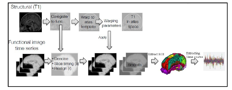 Figure 1.
Employed procedure for ROI signal extraction from raw fMRI data. First, multiple are designed to remove different noises associated with fMRI data including head movement noise, low and high-level noises, gray matter noise and more. Eventually, the time series of 112 anatomical regions are obtained for each subject based on the Harvard-Oxford Atlas.
The preprocessing steps included:
ⅰ. Apply head movement correction.
ⅱ. Apply slice timing correction.
ⅲ. Apply a 3D Gaussian kernel spatial filter with 4 mm3 FWHM (an option in the software above) to increase accuracy of functional image registration to standard space to achieve a better signal to noise ratio (SNR).
ⅳ. Apply high pass filter with 100Hz cut-off frequency to remove low-level noise
ⅴ. Register functional images to T1-weighted images and then register them to MNI152 space using transformations calculated from corresponding anatomical images.
ⅵ. Apply a band pass filter (0.01 Hz - 0.1 Hz) to remove any resting-state BOLD signal associated with neural activity located in the given frequency band.
ⅶ. Filter output data in the previous step by regressing out movement vectors Friston et al. (1996).
ⅷ. Remove unwanted signals such as physiological noise which can be filtered by principal component analysis (Behzadi et al., 2007).
ⅸ. Filter gray matter noise due to scanner heat.
ⅹ. Obtain the time series for 112 anatomical regions for each subject based on the Harvard-Oxford Atlas in the “Extract ROI time courses” tab of the REST software.
Harvard-Oxford atlas is a probabilistic atlas covering 48 cortical and 21 sub-cortical areas. It is derived from structural data and segmentation provided by the Harvard Center for Morphometric Analysis2 (2 https://fsl.fmrib.ox.ac.uk/fsl/fslwiki/Atlases). In this atlas, T1-weighted images of 21 healthy male and 16 healthy female participants (ages 18-50) are individually segmented using semi-automated tools. These images are affine-registered to MNI152 space, and the transforms are then applied to the individual labels. Finally, they are combined across participants to form population probability maps for each label (Karimzadeh et al., 2017).
The summation of the time series from these regions is reformed into a vector (112-by-1) for each subject. These individual vectors are then assembled for each group to give a final 112-by-16 matrix to which the feature extraction method is applied.
Narrowband frequency filtering followed by analytic or complex representation is the conventional approach for IP, frequency, and IE estimation. However, this is highly prone to affect analysis and yield ambiguous values, especially given low SNRs of background activity (Seraj and Sameni, 2017; Sameni and Seraj, 2017). The background activity here refers to the undesired components of the frequency-specific instantaneous measures. To obtain an accurate and unambiguous estimation of IP and IE, a recently developed method was employed (Seraj and Sameni, 2017; Sameni and Seraj, 2017). The method referred to as TFP, is a statistical Monte Carlo based estimation scheme in which infinitesimal perturbations or dithers are added to either the filter or the input signal to generate estimation ensembles (Seraj and Sameni, 2017). In TFP the applied perturbations or dithers are such that they are physiologically irrelevant and the filter’s specification does not change significantly according to the estimation standards (Sameni and Seraj, 2017). The filtering process in TFP is performed as a forward-backward zero-phase approach to avoid any phase distortion. Final IP and IE estimates are obtained from ensemble averaging over all dithered and perturbed ensembles. The rationale behind the TFP is beyond the scope of the current study, but a detailed description can be found in (Seraj and Sameni, 2017; Sameni and Seraj, 2017). To date, TFP has been successfully used in a variety of applications such as BCI (Seraj and Sameni, 2017; Seraj and Karimzadeh, 2017), brain connectivity and synchronization (Sameni and Seraj, 2017; Seraj, 2017) and sleep stage classification (Karimzadeh et al. 2018).
In this study, for both IP/IE estimation and also deriving relevant IP and IE features, we utilized the cerebral signal instantaneous parameters estimation MATLAB toolbox, provided by the authors of (Seraj and Sameni, 2017; Sameni and Seraj, 2017; Seraj, 2017) which is introduced in (Seraj, 2016a) and (Seraj and Mahalingam, 2019) and is available online at (Sameni, 2014). Accordingly, the analytic representation for sequences relating to each brain area in ROI signals extracted from fMRI data is calculated as:
where xi(t) is the sequence in i-th brain area of extracted ROI signal and H{.} represents the Hilbert transform. Using the represented analytic form, IPi IEi for each brain area (i) is estimated as:
Due to the usage of the arctan (.) function, a calculated phase signal might wrap at points where the values cross ± π. Accordingly, a post-processing unwrapping step is required after estimating IP. Fig. 2 shows the estimated IP and IE for each brain area over time-points calculated for the ROI signal extracted from fMRI data of a subject in the dataset employed.
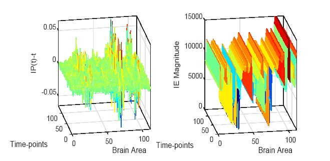 Figure 2.
Estimated IP and IE for each brain area over time-points calculated for the ROI signal extracted from fMRI data of an Alzheimer's patient.
The estimated IP and IE measures for ROI signals derived from the fMRI data obtained from each subject, i.e., AD, MCI, and healthy subjects, are used to extract feature sets. Three different categories of feature such as (1) power, (2) entropy and (3) coherency were calculated for IP and IE to cover almost all aspects of physiological data by using features from both local-scale (relating to one specific brain area) and large-scale (between two widely separated brain areas).
2.4.1 Power feature sets
The energy of the calculated IPs and IEs over time-points for each brain area (i) is used as a measure of power, indicating a local-scale feature set. This set is used to capture the intensity of brain activity in different areas. Accordingly, the differing activities recorded in each cerebral region are putatively discriminative for AD, MCI, and healthy subject data. The energy of ROI signals for each brain area (i) throughout T time-points can be calculated as:
These energy values are stored in vectors of size N, which define the number of brain areas. For each subject, two vectors of length 112 (N = 112) are computed as IP and IE power feature sets.
2.4.2 Entropy feature sets
Entropy indices are directly related to the amount of information embedded in a signal. To capture irregularity and significance of variation of the brain activity within different regions, Shannon entropy can be used as a local-scale feature. Although variance and entropy indices both reveal the information regarding variations and temporal irregularity of the patterns in a signal, the variance is sensitive to the amplitude of values (Sabeti et al., 2009). Accordingly, using the estimated IP and IE values as illustrated in Fig. 3, the Shannon entropy can be calculated for separate brain areas as:
where k is the range of all discrete amplitude values of the signals. Also, pk and lk are the probability of the IPi (t) and IEi (t) signals having the k-th magnitude, respectively. In case that the number of samples in different discretized magnitudes are sufficient, histogram analysis is a proper technique to calculate the probabilities and the entropy.
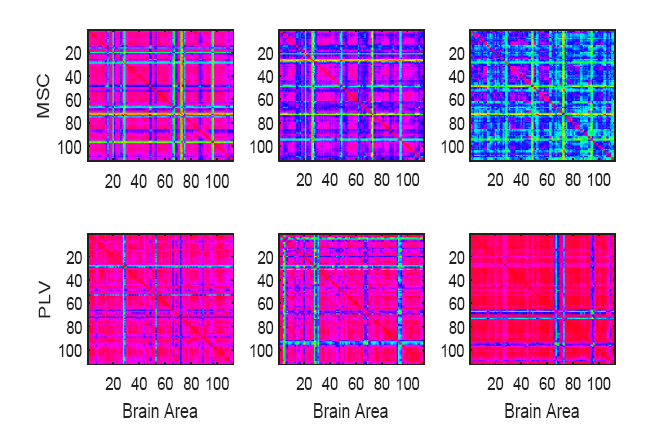 Figure 3.
Sample pairwise PLV and MSC matrices calculated for IP and IE sequences, respectively. From left to right, illustrated matrices belong to Alzheimer's, MCI, and Healthy participants from the utilized dataset. The IPs and IEs are extracted from ROI signals for all (i.e. N = 112) brain areas.
Similarly to the initially obtained power feature sets, the calculated entropies are stored in vectors giving the number of brain areas (N = 112). For each subject, in each of the three classes two vectors (IP and IE) were computed to obtain a second group of sets.
2.4.3 Coherency Feature Sets
Two different, but inherently similar coherency indices, phase-locking value (PLV) and magnitude squared coherence (MSC), are proposed here as suited to investigate the correlation and dependence between the large-scale feature sets of separate brain regions. PLV and MSC feature sets are calculated for the IP and IE sequences extracted from ROI signals, respectively.
PLV is one of the most common measures used in phase analysis.H to describe the phase consistency of two signals (Lachaux et al., 1999). After the estimation of the IP difference between two signals, the local stability of this difference can be quantified by PLV. This stability of IP differences between brain regions (i) and (j) is quantified as:
where T is the length of signals, and the summation is taken over time-points (t).
MSC is employed to investigate the between-region coherency for estimated IE. The usual method for measuring MSC is based on calculating the power spectral densities (PSD) of two signals (Carter et al., 1973). If it is assumed that IEi and IEj are two randomly chosen IE signals from each of two widely separated brain areas (i) and (j), the MSC can be computed as (Seraj, 2016b; Carter et al., 1973):
where $ \mathbb{E}\{.\} $ is the mathematical expectation, and PSDij is the cross-spectrum between instantaneous envelope sequences estimated from ROI signals extracted for the i-th and j-th brain areas (Seraj, 2016b). PLV and MSC are both widely used cerebral synchrony indices, and their values vary between zero and unity. A PLV or MSC value equivalent to unity indicates high signal coherence and synchronicity and vice versa (Seraj, 2016b; Carter et al., 1973).
The coherency of both PLV and MSC is inspected for all possible pairs of the 112 brain areas. This gives a 112-by-112 feature matrix for IPi (t) and IEi (t), respectively. Fig. 3 illustrates sample PLV and MSC matrices calculated for IP and IE sequences of individual participants. This third large-scale category of features contains the coherency and synchrony of the activity of different cerebral areas in fMRI data.
In this step, first, a sequential forward floating feature selection (SFFFS) algorithm is applied to identify the most informative and discriminative sets of features among all six feature sets (one set for each of IP and IE in each of three categories). The feature vector for each class is formed by concatenation of the features calculated from the corresponding IP and IE signals. In this step, each feature set is used solely in a classification process within similar settings and the sets showing the weakest accuracy are left out.
A Student’s t-test is applied to the chosen features and the remaining sets of the former step to select the most relevant and discriminative features within feature-sets. The Student’s t-test is based on the assumption that each class consists of normally distributed features with equal but unknown variances. It tests the null hypothesis that they have equal means (Duda et al., 1973). Accordingly, only features with P -values less than P = 0.05, indicating the confidence level at which the null hypothesis may be rejected, are included in the classification stage.
The remaining features are gathered and concatenated for each of the three classes, and the corresponding labels are assigned. The AD subjects, MCI and healthy participants are labeled as 1, 2 and 3 respectively. All selected feature sets were combined, and a K-NN classifier performed final discrimination between the three classes. Various values of K were tested (K = 1, 5, 10 and 15). K = 5 showed the best performance and was chosen for all levels of classification (i.e. feature selection with SFFFS). The data of 30 subjects (i.e. 10 of each class) were chosen at random for testing while the remaining 81 were used to train the classifier. Accordingly, the classifier was trained with an entire combined set of features with a single label and returned a single value, i.e. 1, 2 or 3.
The results of classifying AD, MCI and healthy subjects by the combination of all chosen features were evaluated by calculating four standard classification performance indicators, accuracy (AC), precision (PR), specificity (SP) and sensitivity (SE). Initially, the result of feature selection through significance tests is reviewed. Significance tests were performed for all three possible cases, i.e., AD vs. MCI, AD vs. healthy and MCI vs. healthy and results are given in Fig. 4. The confidence level for the rejection of the null hypothesis was 5% (P-value < 0.05). As can be seen, approximately 80% to 90% of calculated features were confirmed to be statistically significant.
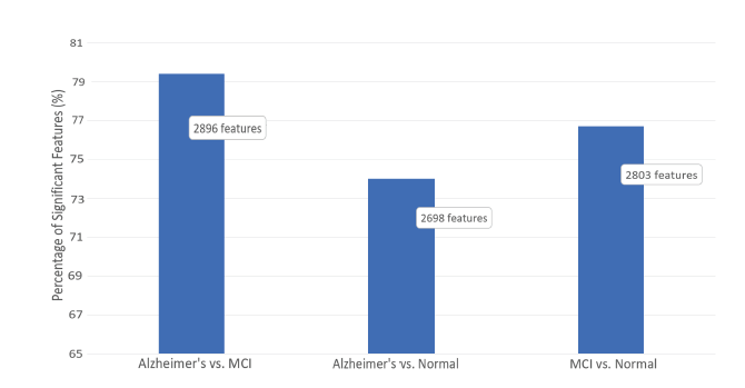 Figure 4.
Percentage of statistically significant features selected by Student's t-test to be involved in the classification stage. As shown, on average only around 75% of the extracted features have been selected as significant and were used in the classification stage.
The selected features were then classified by the use of a 5-NN classifier as described previously. Classification correctly labeled 21 of the 30 test subjects. This resulted in an average accuracy of all classes of 80.1%. The confusion matrix of this evaluation is given in Table 2.
| Truth Data | Precision | ||||
|---|---|---|---|---|---|
| Alzheimer's | MCI | Healthy | |||
| Classifier | Alzheimer's | 8 | 3 | 1 | 66.7% |
| MCI | 2 | 5 | 1 | 62.5% | |
| Healthy | 0 | 2 | 8 | 80.0% | |
| Recall (Sensitivity) | 80.0% | 50.0% | 80.0% | Overall Accuracy = 80.1% | |
The accuracy, precision, specificity, and sensitivity of the proposed features given in Table 2 are illustrated in Fig. 5 both for each class and in total. AC, PR, SP, and SE are calculated, respectively, as:
The overall accuracy, precision, specificity, and sensitivity are then computed as the average AC, PR, SP, and SE of all classes, respectively.
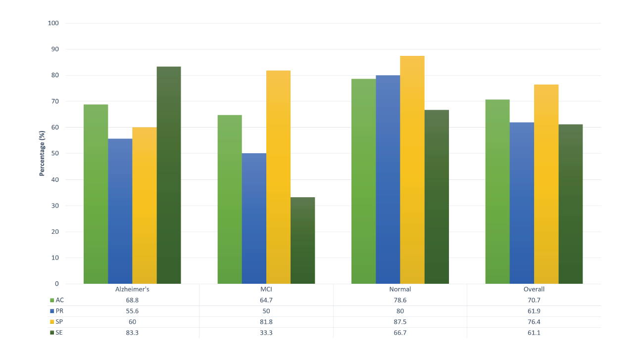 Figure 5.
Obtained accuracy (AC), precision (PR), specificity (SP), and sensitivity (SE) for each of three classes and the overall case. The proposed methodology shows relatively significant sensitivity to the distinction of the Alzheimer's and Normal cases while demonstrating high specificity for the MCI cases.
As depicted in Fig. 5, the classes belonging to the AD subjects and healthy participants show the highest accuracy, whereas, the MCI case is given lower values. Table 2 reports that eight of nine misclassifications were somehow related to the MCI category. Moreover, three of the MCI cases were mistaken as AD subjects which are taken to show the close similarity of these two classes. Consequently, although eight of ten AD subjects were identified correctly, SP and PR were not relatively high for that class (when compared with the healthy category). The proposed IP and IE features generally appear to give significant results. However, further investigation is required to improve the classification rate of MCI subjects.
Detection of AD at an early stage is significantly important for the application of appropriate treatments. Thus, new trends in this domain are moving toward the use of more efficient algorithms to distinguish healthy subjects from AD patients. Here, an algorithm is introduced that by use of fMRI data could efficiently classify subjects as either healthy individuals or those with different stages of AD. A more recent and related report to this one is that of (Wang et al., 2018). They proposed an approach based on previous observations that shows some parts of default mode network at resting-state fMRI lose their functional connectivity in AD. These ROI’s were extracted from fMRI data and their correlation coefficients computed. In that case, linear discriminant analysis was employed to distinguish between AD, MCI and healthy subjects and an AdaBoost classifier was applied to distinguish AD patients from healthy subjects, Although, their results showed good performance by their analytic approach even in the case of limited samples for AD classification, misclassification of MCI subjects was still high. Moreover, their algorithm both used a complex classifier for one-dimensional data which may not be appropriate in the given circumstances and was highly dependent on the ROI selection step.
In the study reported here, an alternative approach was developed. It is based on extracting new features and selecting the most discriminative from among AD, MCI, and healthy subjects. The proposed algorithm does not require a complex classifier and any simple classification tool such as K-NN can be efficiently employed. Additionally, for the first time, new features are introduced, including IP and IE sequences of ROI signals, extracted from fMRI data, where the selected ROIs are based on the Harvard-Oxford probabilistic brain atlas. The most informative sets of these features are identified by SFFFS. Observation showed that this new set of features efficiently both represents the characteristics of fMRI data and discriminates different stages of AD. Although, as shown in Fig. 5, separating MCI patients has the least accuracy, the algorithm mostly mistakes them for AD subjects and not healthy subjects, which is clinically more acceptable. This is inevitable to some extent due to variations between the brains of subjects such as aggregation of protein fragment beta-amyloid outside of neurons and abnormally accumulated protein tau (tau tangles) inside neurons, both of which are similar in MCI and AD subjects when compared with healthy individuals1. Generally, the results obtained by application of the proposed algorithm to fMRI data show good performance and could be a promising approach for clinical applications.
Although performance of the chosen features and their specific contributions to overall performance might appear to be black-boxed, a simple feature analysis test through which features are added and analyzed step-by-step (i.e., add a feature set while removing the rest or freezing one set of features while varying another) reveals to some extent those features that are the most discriminative for the application of interest. Here, all the feature categories introduced were based on IP and IE notions of fMRI data. It is left to the reader to decide which features to test and use according to data availability and the given application. MATLAB implementations are available for the fundamental methods of IP and IE extraction, MSC score, and PLV analysis to help with testing and analysis and facilitate the reproducibility of this study, in (Seraj and Mahalingam, 2019) and (Seraj, 2016a).
ES proposed the algorithms and was responsible for data analysis and classification. NS was responsible for data preparation and preprocessing and also writing the Introduction and Preprocessing sections. ES wrote the rest of the manuscript. MY was in charge of general research guidelines and idea development. All authors contributed to editorial changes in the manuscript. All authors read and approved the final manuscript.
This research has been supported by the Cognitive Sciences and Technologies Council of Iran (COGC), under grant number 2250.
The authors declare no competing interests.