
- Academic Editor
Background: As an objective method to detect the neural electrical activity of the brain, electroencephalography (EEG) has been successfully applied to detect major depressive disorder (MDD). However, the performance of the detection algorithm is directly affected by the selection of EEG channels and brain regions. Methods: To solve the aforementioned problems, nonlinear feature Lempel–Ziv complexity (LZC) and frequency domain feature power spectral density (PSD) were extracted to analyze the EEG signals. Additionally, effects of different brain regions and region combinations on detecting MDD were studied with eyes closed and opened in a resting state. Results: The mean LZC of patients with MDD was higher than that of the control group, and the mean PSD of patients with MDD was generally lower than that of the control group. The temporal region is the best brain region for MDD detection with a detection accuracy of 87.4%. The best multi brain regions combination had a detection accuracy of 92.4% and was made up of the frontal, temporal, and central brain regions. Conclusions: This paper validates the effectiveness of multiple brain regions in detecting MDD. It provides new ideas for exploring the pathology of MDD and innovative methods of diagnosis and treatment.
Depression is one of the most common mental illnesses, and the number of patients increases yearly. According to a survey report by the World Health Organization, the number of patients with depression has reached 320 million worldwide [1]. With the increasing number of patients with depression, social problems, such as insufficient medical resources for diagnosing and treating depression follow. At present, the diagnosis of depression in clinical settings mostly relies on depression scales and clinical manifestations, which are highly subjective and prone to problems such as missed diagnosis and misdiagnosis [2]. An effective way to reflect the neural electrical activity of the brain is through electroencephalography (EEG), a noninvasive, quick, and simple clinical diagnostic tool. Numerous studies have demonstrated that depression is a psychiatric disorder associated with dysfunction of the amygdala, thalamus, and anterior cingulate gyrus [3, 4, 5]. Furthermore, abnormal brain activity can cause changes in EEG [6, 7], so by observing the changes in EEG in major depressive disorder (MDD), we can deeply study its pathogenesis and explore effective diagnosis and treatment methods.
To improve the accuracy of using EEG signals to identify patients with MDD, researchers have conducted much research on this. The alpha and theta bands of the EEG signals of patients with MDD differ from those of normal people, according to some researchers who have analyzed the EEG in the time and frequency domains [8, 9]. However, due to the nonlinear dynamic characteristics of EEG, using simple linear methods to describe the nonlinear, nonstationary, and chaotic complex dynamic changes of EEG is difficult [10, 11]. Nonlinear methods are now being used in an increasing number of studies to analyze the EEG signals of patients with MDD. RoSchke et al. [12] analyzed the sleep EEG signals of depression and extracted the Lyapunov index and the correlation dimension D2 to distinguish patients with MDD. Hasanzadeh et al. [13] used multiple nonlinear feature fusion to detect patients with depression treated with repetitive transcranial magnetic stimulation (rTMS) and achieved a classification accuracy of 91.3%. Using the k-Nearest Neighbors (KNN) model, Bai et al. [14] classified the complexity features of the gamma frequency band extracted from the nonlinear domain with an accuracy of 79.63%. The fractal dimension of the beta frequency band was extracted and obtained an accuracy of 65.94% using the random forest classifier. EEG contains a large amount of information about neural electrical activity. The correlation of brain regions plays a significant role in detecting depression in addition to the characteristics of each channel. Wang et al. [15] found that the temporal lobe area was significantly different between patients with MDD and people without MDD through brain topography, verifying that the temporal lobe area was an important brain area for distinguishing patients with MDD from people without MDD. This finding was consistent with the interpretation of pathology by the data provider [16]. Mohan et al. [17] used an artificial neural network to distinguish patients with depression from people without depression in each brain region. Finally, they found that the central brain region (C3 and C4) was the best brain region to identify depression. Mahato et al. [18] studied the linear and nonlinear characteristics of EEG signals of patients with depression. They found that depression had different impacts on the left and right hemispheres and manifested differently in various brain regions. Heo et al. [19] found that the symptoms of depression and anxiety in patients with depression may be related to the asymmetry of theta waves from the frontal to the central brain area. Jiang et al. [20] divided all brain regions (from the frontal to the occipital areas) into three parts for experiments. They proved that the information between brain regions is very useful for improving depression recognition accuracy. Sun et al. [21] proposed a multilayer brain functional connectivity network. They found that the brain functional connectivity network’s right frontal and temporal lobe regions in patients with MDD have connectivity defects. As a result, brain region-related features in EEG signals are crucial for understanding the pathology of depression and improving the accuracy of depression detection.
In this paper, the EEG signals of patients with MDD and healthy control groups were studied with eyes closed (EC) state and opened (EO) state in resting. Through the fusion analysis of the nonlinear characteristic Lempel–Ziv complexity (LZC) and the frequency domain characteristic power spectral density (PSD) of the EEG signal, we investigated the effects of different brain regions and brain region combinations on the detection of patients with MDD to improve the detection accuracy of patients with MDD. The best brain regions and patterns of brain region pairings for detecting patients with MDD using EEG were confirmed.
The data used in this paper were from the public dataset MPHC
(https://figshare.com/articles/EEG_Data_New/%204244171) [16], which recruited
34 patients with MDD (17 men and 17 women, mean age = 40.3
In this paper, the placement of brain electrodes on the scalp followed the International 10–20 system [23]. EEG data were gathered using an EEG cap with 19 electrode channels.
The preprocessing of the EEG data in this study was conducted using EEGLAB (EEGLAB2022.1, Swartz Center for Computational Neuroscience, San Diego, CA, USA). The electrodes are positioned using the electrode system after each set of EC and EO data has been imported. Then, the data were filtered and a finite-length unit impulse response (finite impulse response) filter was used to perform high-pass filtering at 0.1 Hz. Low-pass filtering at 45 Hz was introduced to reduce the interference caused by the power frequency. After carefully examining the waveform, the bad channel was manually removed, and its average value was substituted with the channels close to it. Independent component analysis (ICA) can effectively extract and remove artifacts produced by eye and head movements [24]. The collected raw EEG data shown various artifacts and valid EEG signals. These data are not dependent on one another and typically follow a non-Gaussian distribution [25], making it possible to divide them into independent components using ICA. This study uses EEGLAB’s ICA tool, which uses a “runica” algorithm with default settings, calculates independent components based on the actual number of channels, and removes artifact components by observing brain topography and time domain chromatograms, and power spectra.
After data preprocessing, some subjects lacked EC or EO data, and data with a short data lengths were removed. Data of EO and EC for 4 min each were collected from 25 healthy controls and 24 patients with MDD. We segmented all the data with a length of 10 s and finally obtained 576 and 576 segments with EC and EO for patients with depression, respectively, whereas the control group had 600 and 600 segments with EC and EO, respectively.
The frequency domain feature selected in this paper is PSD [26], with a sampling
frequency of 256 Hz and a hanging window. First, the full-band PSD value of each
electrode was calculated. Lempel and Ziv [27] proposed the LZC feature, and
Kaspar [28] later designed it as a simple and user-friendly program. Before
calculating the complexity, the EEG signal X(x(1),
x(2), …, x(n)) must be transformed into a
binary sequence Y(s(1), s(2), …,
s(n)), where n is the total number of sampling points
of the signal, 1
In this study, the threshold m was set to be the median value of the EEG because the median value performs better than the average value when there are abnormal values in the signal [29]. Then, we traverse all characters of sequence Y to obtain the complexity c(n) of sequence Y.
Lempel and Ziv [27] have shown that the upper bound on c(n) is b(n). a is the number of coarse-grained segments.
In this paper, the EEG signal sequence is binarized, so a = 2. To avoid changes caused by the length of the sequence segment, it is necessary to perform a normalization operation on c(n); the operation is as follows:
In principle, LZC represents the rate at which new patterns appear in the EEG signals. The normalized LZC is higher, indicating that the number of new patterns in EEG is large and that the brain activity is more complex. Because brain regions discharge irregularly, the EEG sequence tends to be more random.
Support vector machine (SVM) is a classic model for binary classification. This paper selects SVM as the classifier to classify the extracted features from the preprocessed data with EC and EO with a “linear” kernel and the BoxConstraint of 1.
In the cross-subject experiment, healthy individuals and patients with depression were divided into five groups. One random group was selected from all groups, and the feature matrix of the selected groups was used as the test set, whereas the feature matrix of the remaining groups was used as the training set. That is, samples from the same person cannot be used simultaneously as training and test data. The results were averaged after 100 times fivefold cross-validations.
In the binary classification, according to the predicted situation of the sample and the actual label, it can be divided into true positive (TP), false positive (FP), true negative (TN), and false negative (FN). Then, the confusion matrix of the binary classification, shown in Table 1. Patients with MDD were positive, and controls were negative. TP is the patients with MDD and predicted as MDD. FP is the control group and predicted as patients with MDD. TN is the control group and predicted as control. FN is the patients with MDD and predicted as control.
| Predicted: Positive | Predicted: Negative | |
| Actual: Positive | TP | FN |
| Actual: Negative | FP | TN |
TP, true positive; FP, false positive; TN, true negative; FN, false negative.
This matrix can obtain its sensitivity, specificity, accuracy, and other indicators. We need to examine a model from various indicators to assess its quality. Therefore, in addition to comparing the model’s accuracy, it is often necessary to comprehensively consider the model along with indicators such as sensitivity and specificity. The specific calculation formula is as follows:
According to the International 10–20 system, the brain regions are divided, as shown in Table 2.
| Brain region | Channels | |
| 1 | Frontal | Fp1, Fp2, F3, and F4 |
| 2 | Temporal | F7, F8, T3, T4, T5, and T6 |
| 3 | Central | C3, C4, Fz, Cz, and Pz |
| 4 | Parietal and Occipital | P3, P4, O1, and O2 |
According to the 10–20 system, electrodes can be divided into frontal, temporal, central, and occipital brain regions, which can be better analyzed by the brain region. First, we construct feature matrices for specific brain regions. The splicing of a feature matrix of the brain regions results in a feature matrix of a combination of multiple brain regions. For example, B1 and B2 are the corresponding feature matrices of two brain regions (The columns of the matrix represent the proposed features of a piece of data), then the feature matrix after the combination of brain regions is (B1; B2).
After the LZC and PSD features are extracted, the average value is obtained for analysis. The topographic maps of the control group and the patients with MDD in EC state are shown in (a) and (b) in Fig. 1, respectively, whereas the topographic maps of the control group and the patients with MDD in EO state are shown in (c) and (d) in Fig. 1, respectively.
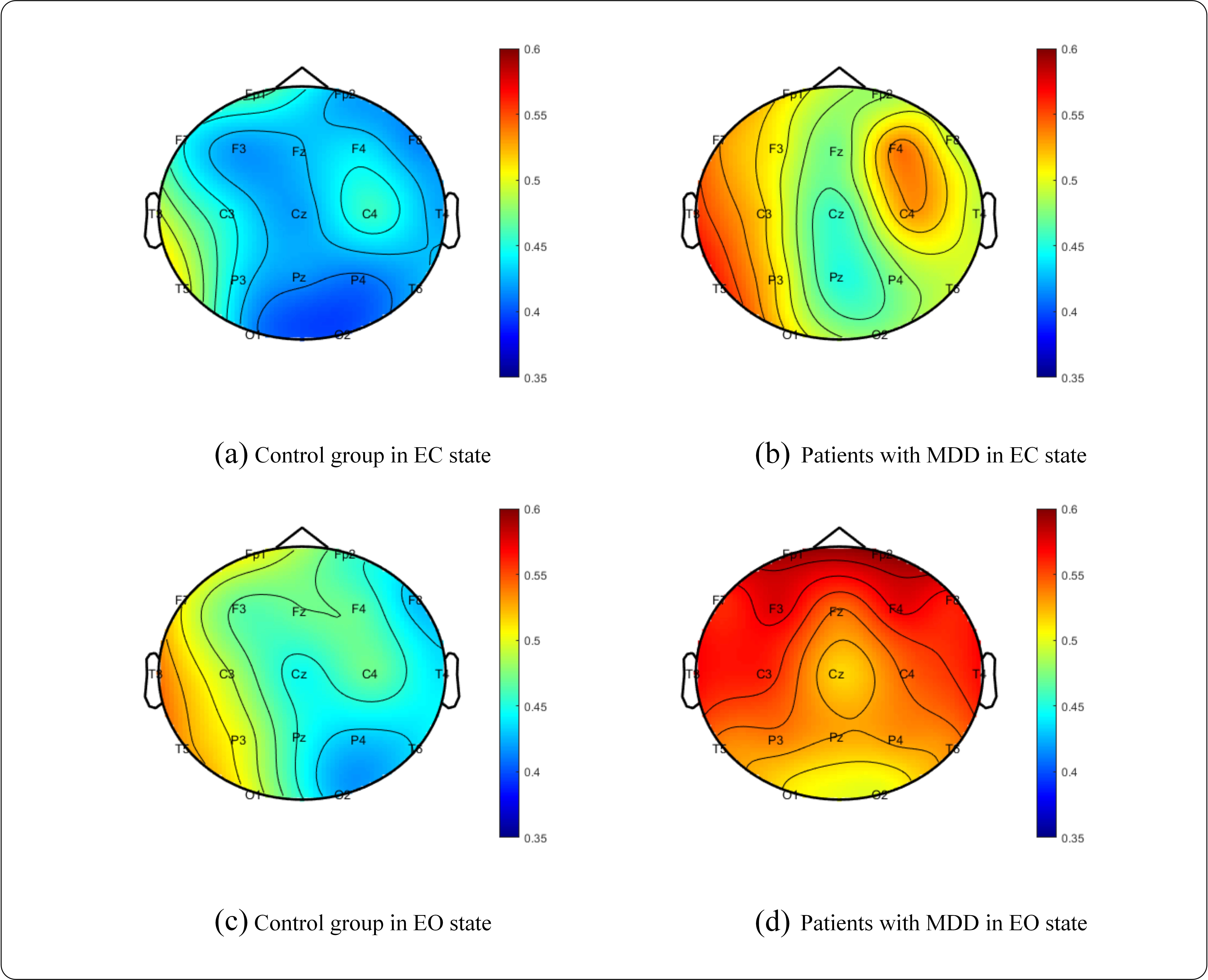 Fig. 1.
Brain topography of the LZC mean. (a) Control group in EC. (b) MDD in EC. (c) Control group in EO. (d) MDD in EO. EC, eyes closed; MDD, major depressive disorder; EO, eyes opened.
From Fig. 1, we can see that the mean LZC value of the patients with MDD is higher than that of the control group, indicating that the irregular discharge of brain regions and the complexity of brain activity in patients with MDD are higher than those in the control group. Additionally, it can be seen that the mean LZC value of the control group and patients with MDD in EO state is higher than that in EC state, indicating that the brain activity in the EO state is more complex than that in the EC state.
From Fig. 2, we can see that the mean PSD of patients with MDD is lower than that of the control group, indicating that the activation degree of the brain of patients with MDD is lower than that of the control group, which corresponds to the findings of the study by Lechinger et al. [30]. And, as can be seen, the mean PSD of the control group and patients with MDD in the EO state is higher than that in the EC state, indicating that the EO state has higher brain activity than the EC state.
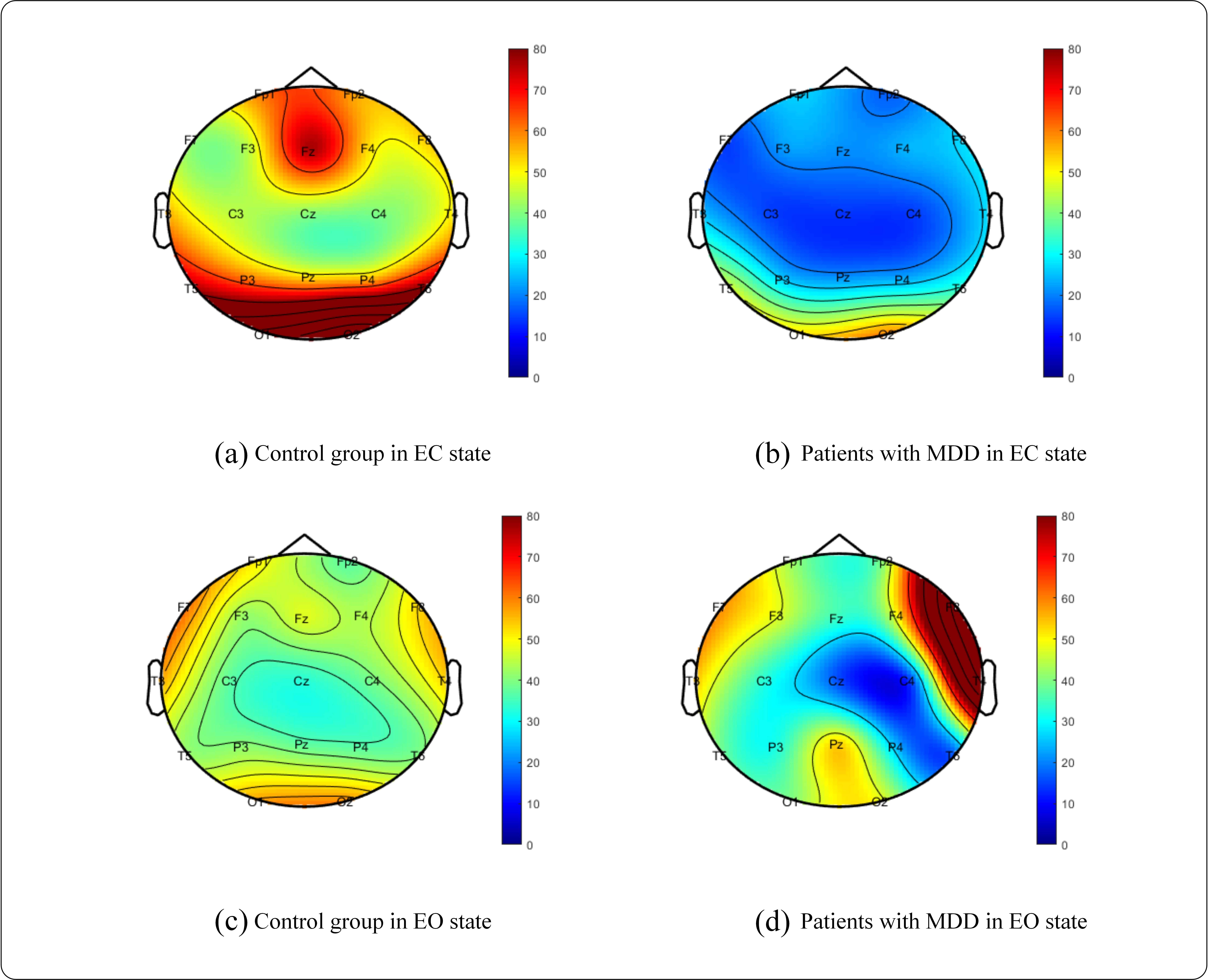 Fig. 2.
Brain topography of the PSD mean. (a) Control group in EC, (b) MDD in EC, (c) Control group in EO, (d) MDD in EO.
Tables 3,4 demonstrate the detection performance of EC and EO states,
respectively. According to Tables 3,4, using the nonlinear feature LZC and
the frequency domain feature PSD together has a better detection effect than
using only the LZC or PSD feature in both the EC and EO states. Furthermore, the
highest detection accuracy rate of multiple features can reach 91.0%, which is
much higher than that of one feature. This result shows that these two features
have complementary roles in identifying MDD and that subsequent studies use multi
feature fusion for experiments. In this paper, t-test is used to test
the differences between patients with MDD and control group in various feature
matrices. As we can see from Tables 3,4, we calculated the p-value of
LZC, PSD and LZC + PSD between two groups in the EC and EO states respectively,
all features show significant differences with p
| Sensitivity (%) | Specificity (%) | Accuracy (%) | p-value | |
| LZC | 76.9 | 74.2 | 75.6 | |
| PSD | 74.2 | 70.0 | 72.1 | 0.036 |
| LZC + PSD | 78.9 | 78.3 | 78.6 |
LZC, Lempel–Ziv complexity; PSD, power spectral density.
| Sensitivity (%) | Specificity (%) | Accuracy (%) | p-value | |
| LZC | 86.7 | 89.2 | 87.9 | |
| PSD | 89.4 | 68.9 | 79.2 | 0.021 |
| LZC + PSD | 92.8 | 89.2 | 91.0 |
According to the division of brain regions in Table 2, the fusion features extracted from the channels of each brain region are used as feature sets, a two-dimensional matrix of features of each brain region is constructed, and SVM is used for classification. For example, in EC and EO states, the classification results of each single brain area are shown in Tables 5,6. In Tables 5,6 and Figs. 3,4, F, T, C, and O stand for the frontal, temporal, central, parietal and occipital lobes, respectively, and ALL stands for the entire brain region.
| Brain region | Sensitivity (%) | Specificity (%) | Accuracy (%) | p-value |
| F | 72.2 | 74.2 | 73.2 | |
| T | 80.3 | 78.6 | 79.4 | |
| C | 78.9 | 70.0 | 74.4 | |
| O | 72.2 | 71.9 | 72.1 | 0.015 |
F, frontal lobes; T, temporal lobes; C, central lobes; O, occipital lobes.
| Brain region | Sensitivity (%) | Specificity (%) | Accuracy (%) | p-value |
| F | 79.5 | 79.8 | 79.6 | |
| T | 84.7 | 90.0 | 87.4 | |
| C | 83.6 | 70.6 | 77.1 | |
| O | 83.6 | 77.2 | 80.4 |
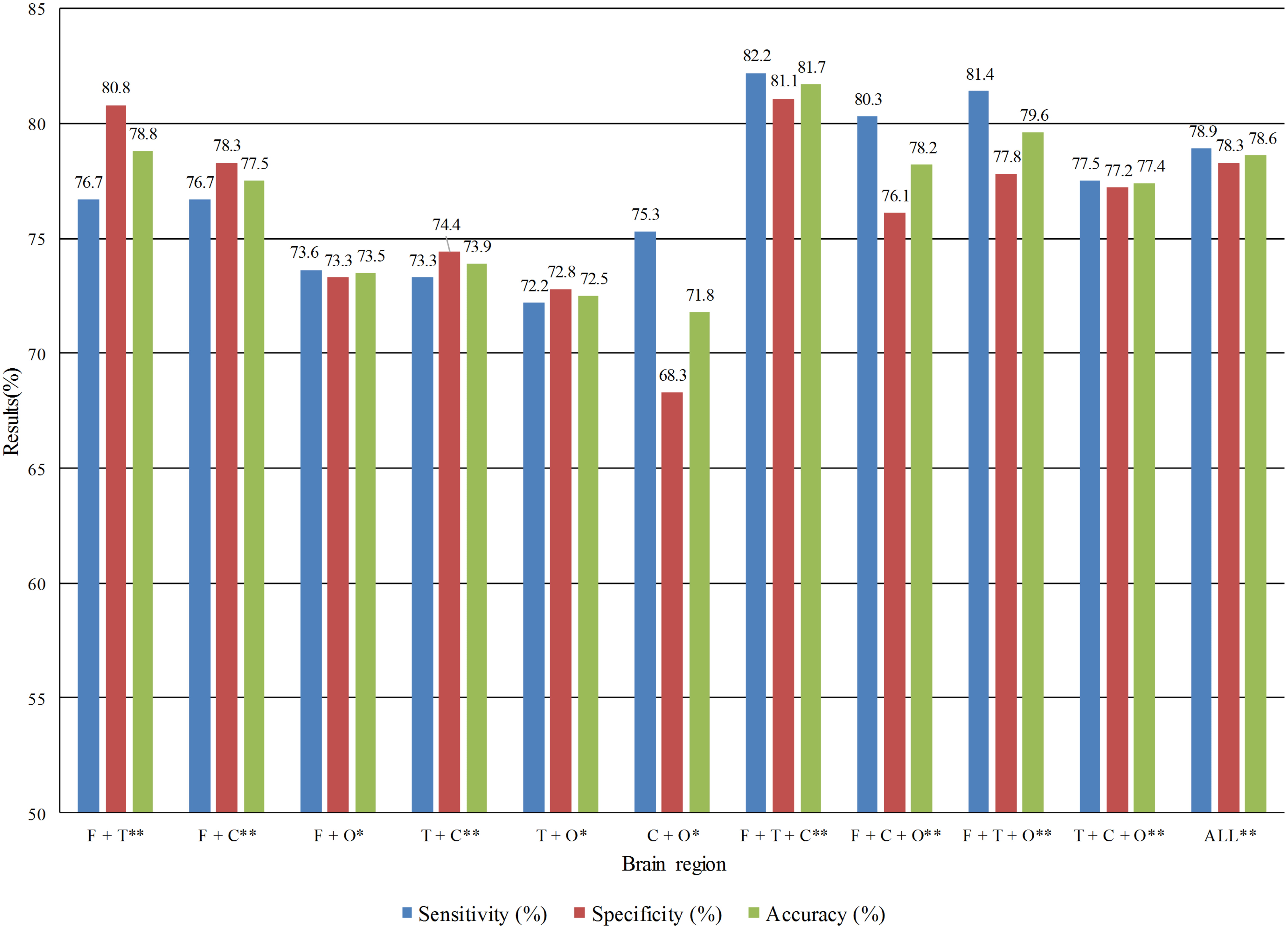 Fig. 3.
Detection performance of multi brain regions combination in the
eyes closed state. *Statistical difference significance between two groups with
p
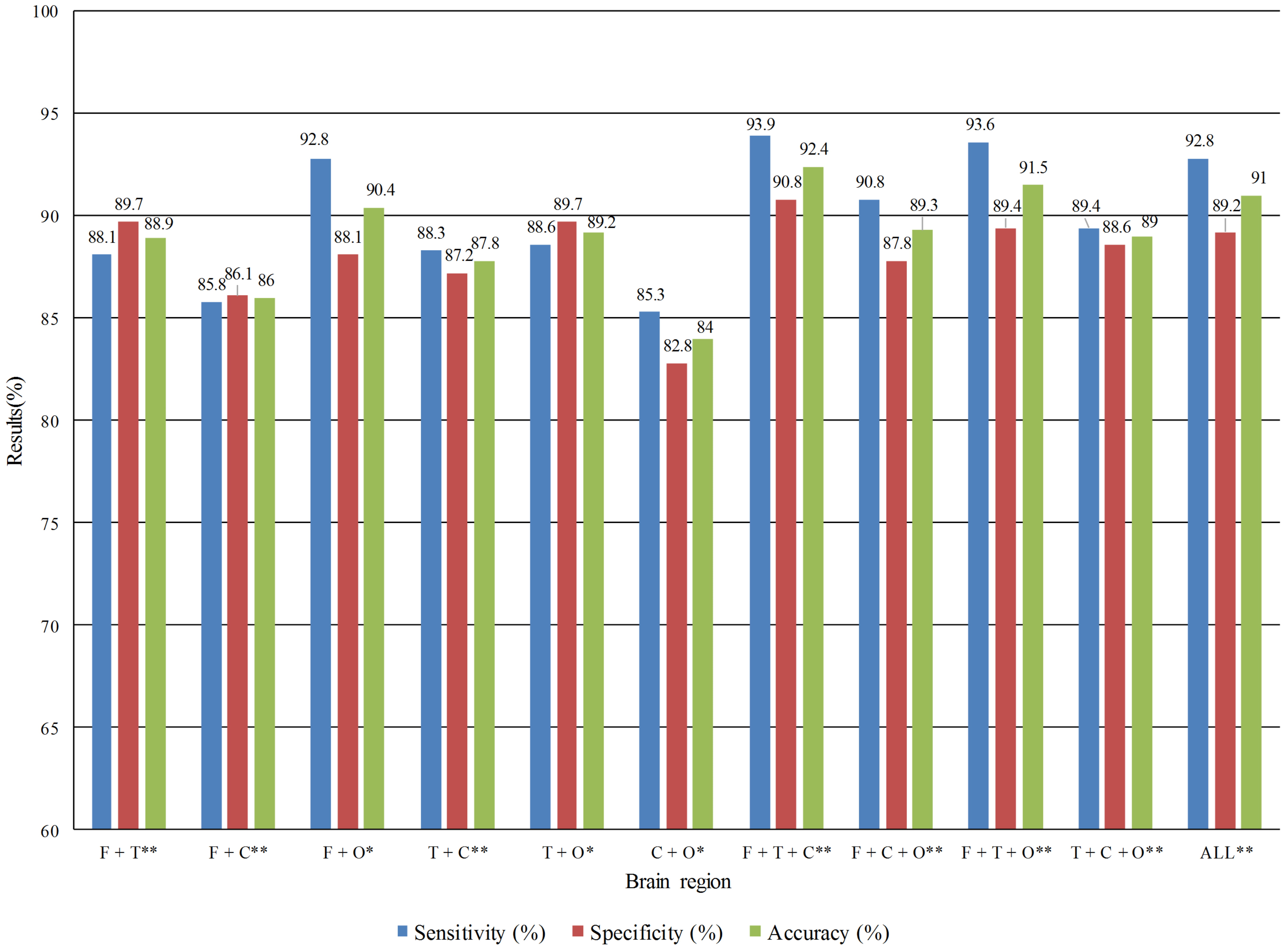 Fig. 4.
Detection performance of multi brain regions combination in the
eyes opened state. *Statistical difference significance between two groups with
p
Tables 5,6 shows that in the EC state, the best effect was in the temporal
lobe region, with a sensitivity of 80.3%, specificity of 78.6%, and accuracy of
79.4%. In the EO state, the best effect was also in the temporal lobe region,
with sensitivity of 84.7%, specificity of 90.0%, and accuracy of 87.4%. This
confirms the temporal significance for MDD recognition and is consistent with how
the data providers of this study interpreted the pathology. We used t-tests on
the feature matrices of single brain region between patients with MDD and control
group and found that the O brain region shows significance with p
We tried merging two or three brain regions or the feature matrix of the three brain regions channels and used SVM for classification. For example, in EC and EO states, the combined detection effects of each multi brain regions are shown in Figs. 3,4.
From Figs. 3,4, it was found that the combination of frontal, temporal, and
central lobe regions performed the best in both EC and EO states, with
sensitivity, specificity, and accuracy rates of 82.2%, 81.1%, and 81.7% in the
EC state and 93.9%, 90.8%, and 92.4% in the EO state, respectively.
Additionally, we discovered that the frontal, temporal, and central lobe regions
combination increased accuracy by 5% over the best single brain region. The best
multi brain regions combination compared with the full brain, the accuracy is
1.4% higher, the specificity is 1.6%, and the sensitivity is 1.1%. We used
t-tests on the feature matrices of various brain region combinations
between patients with MDD and control group and found that the frontal,
temporal, and central region combinations show significant differences with
p
The confusion matrix of optimal combination is shown in Fig. 5. From the confusion matrix, we can observe that the proposed model in this paper owns well sensitivity for detecting MDD patients.
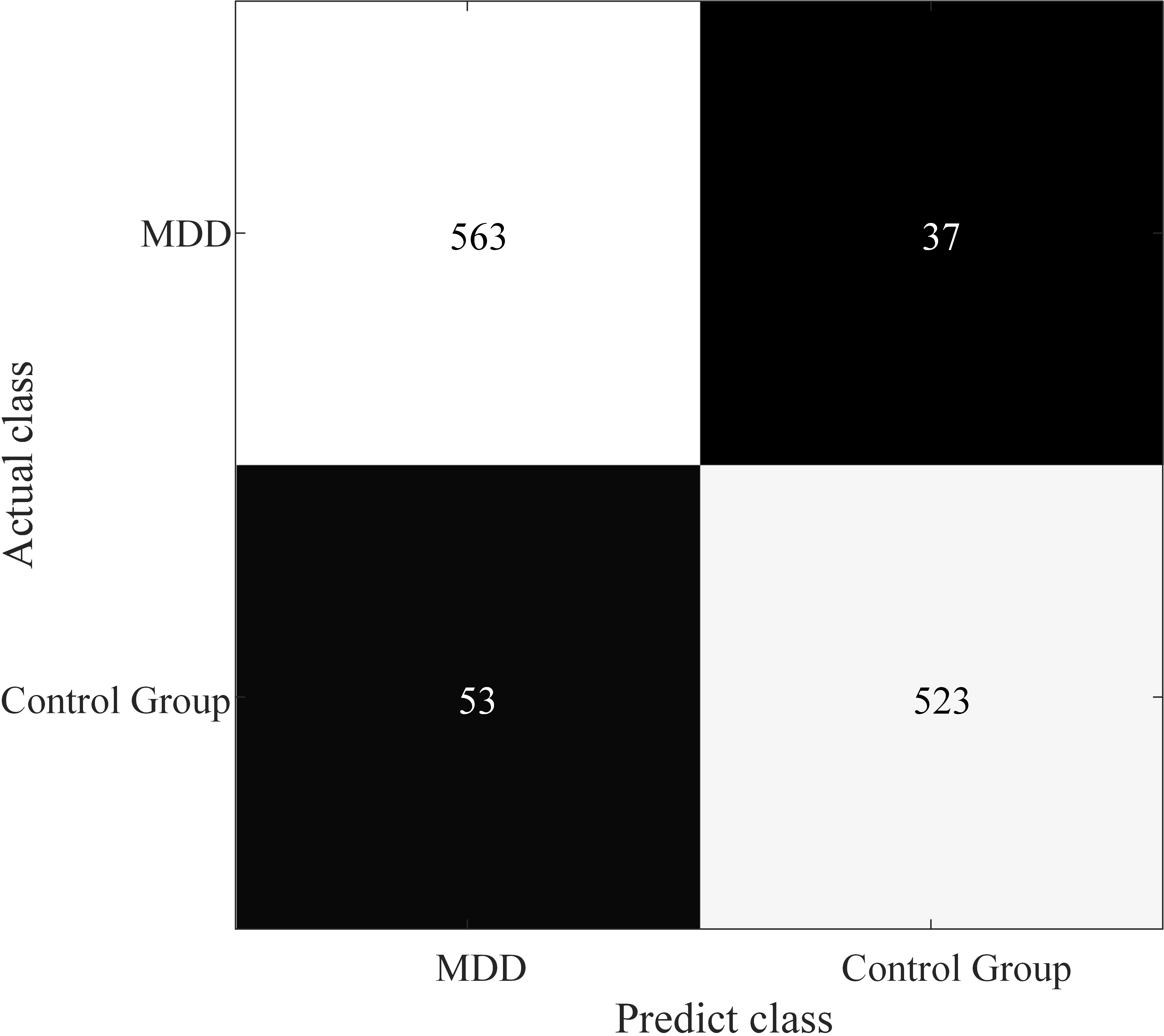 Fig. 5.
Confusion matrix for optimal combination of brain regions.
According to this study, in the case of a multi brain combination, the EO state is more likely to be recognized than the EC state. This may be because the functional connection strength of the brain in the EO state is higher than that in the EC state. In the case of a combination of multiple brain regions, the difference between the brain regions of patients with MDD and control group is more realistically expressed [31].
This paper found that the temporal lobe region had the best effect among the single brain regions. The combination of frontal, temporal, and central lobe regions combination is best in multi brain regions analysis. This may be related to the hippocampus and amygdala in the brain’s limbic system. The amygdala and the hippocampus, which are involved in memory and emotional responses, are found in the dorsomedial region of the anterior temporal lobe region and are located below the hypothalamus. Correlation studies have shown that the degree of connectivity of amygdala-related functional connectivity is associated with depression duration [32]. Depression is associated with the anterior cingulate gyrus and the orbital prefrontal cortex in the frontal lobe region and the superior temporal gyrus, hippocampus, and amygdala in the temporal lobe region [33]. This research reveals that the frontal, temporal, and central brain regions that worked best together were the hippocampus and amygdala, frequently studied in MDD research. These brain regions will have reference significance for subsequent MDD research.
This study found that the mean LZC and PSD values of EEG signals in the resting EO state and resting EC state of patients with MDD differed from those of the control group. When the detection of results from the two experimental paradigms are compared, we observed that the detection effect of the resting EO state is generally higher than that of the resting EC state. From the test results, the accuracy rate of the combined brain regions is improved significantly. Among them, the channel combination of the frontal, temporal, and central brain regions is better than single brain regions, multi brain regions combinations, and the full brain. It can achieve 92.4% cross-subject recognition accuracy on the public dataset. Additionally, we discovered that the ideal combination of brain regions matches the pertinent brain regions currently being studied in the pathology of MDD. This study will provide a reference for future research on the auxiliary detection of brain diseases. The limitation is that we used public EEG datasets. Some information about EEG collecting was missing, which will be an obstacle to analyzing the inner mechanism and further verification.
The datasets used and analyzed during the current study are available from the corresponding author on reasonable request.
JY, ZZ, PX and XL designed the research study. JY and ZZ performed the research. PX and XL provided help and advice on the experiments. ZZ analyzed the data. All authors contributed to editorial changes in the manuscript. All authors read and approved the final manuscript. All authors have participated sufficiently in the work and agreed to be accountable for all aspects of the work.
Not applicable.
We would like to thank the data providers for providing data for this study.
This work was supported by the National Natural Science Foundation of China (62006067, U20A20224), Natural Science Foundation of Hebei Province (F2021201008), Key Projects of Science and Technology Research in Hebei Higher Education Institutions (ZD2021013) and Foundation of President of Hebei University (XZJJ201907).
The authors declare no conflict of interest.
Publisher’s Note: IMR Press stays neutral with regard to jurisdictional claims in published maps and institutional affiliations.