
- Academic Editor
Background: There are several antibiotic resistance genes (ARG) for the
Escherichia coli (E. coli) bacteria that cause urinary tract infections
(UTI), and it is therefore important to identify these ARG. Artificial
Intelligence (AI) has been used previously in the field of gene expression data,
but never adopted for the detection and classification of bacterial ARG. We
hypothesize, if the data is correctly conferred, right features are selected, and
Deep Learning (DL) classification models are optimized, then (i) non-linear DL
models would perform better than Machine Learning (ML) models, (ii) leads to higher accuracy, (iii) can identify the hub genes,
and, (iv) can identify gene pathways accurately. We have therefore
designed aiGeneR, the first of its kind system that uses DL-based models
to identify ARG in E. coli in gene expression data.
Methodology: The aiGeneR consists of a tandem connection of quality
control embedded with feature extraction and AI-based classification of ARG. We
adopted a cross-validation approach to evaluate the performance of aiGeneR using
accuracy, precision, recall, and F1-score. Further, we analyzed the effect of
sample size ensuring generalization of models and compare against the power
analysis. The aiGeneR was validated scientifically and biologically for hub genes
and pathways. We benchmarked aiGeneR against two linear and two other non-linear
AI models. Results: The aiGeneR identifies tetM (an ARG) and showed an
accuracy of 93% with area under the curve (AUC) of 0.99 (p
Escherichia coli (E. coli) is a bacterium that is frequently discovered in both human and animal gastrointestinal tracts. While E. coli is mostly not harmful, some strains can cause diseases, such as urinary tract infections (UTI) [1, 2]. These infections that can affect the kidneys, bladder, ureters, and urethra, as well as other parts of the urinary system [3]. One of the most frequent bacteria that cause UTI, especially in women, is E. coli. Lower abdomen or back pain, frequent urination, murky or bloody urine, and pain during urination are all signs of an E. coli-related UTI [4, 5].
E. coli and other bacteria are becoming increasingly resistant to antibiotics. When bacteria learn to counteract antibiotic effects, antibiotic resistance arises, making infections more challenging to treat. By several methods, including genetic changes and the exchange of resistance genes across bacteria, E. coli can develop antibiotic resistance [6, 7]. Antibiotic resistance can also be brought on by the overuse and abuse of antibiotics. Many E. coli strains exhibit resistance to one or more drugs. As a result, treating E. coli infections may become more challenging and necessitate the use of different antibiotics or lengthier treatment regimens [8].
Antimicrobial resistance (AMR), which includes the concept of antibiotic resistance, is an increasing concern to healthcare systems around the globe and places a significant financial burden on international healthcare systems [9]. AMR was ranked fifth among the top 10 global health hazards by the World Health Organization (WHO) in 2019 [10]. Antibiotic resistance is a significant public health issue because it reduces the efficacy of several antibiotics that are commonly used to treat bacterial infections. Each year in United States, 2.8 million individuals get affected, resulting in 35,000 deaths [11]. The death count in the European region due to AMR in various infected agents for the year 2019 is shown in Fig. 1. It is observed that the death due to UTI is 48,700 which is 5% of the total deaths [11, 12, 13].
 Fig. 1.
Statistics of deaths due to AMR in Europe (2019) [11]. AMR, Antimicrobial resistance; CNC, Certified Nutrition Consultant; LRI, Lower respiratory infection; iNTS, invasive non-typhoidal Salmonella.
Antibiotic resistance genes (ARG) adopt various biological processes and are responsible for making a bacterium to defend the drug. Identifying the ARG is the most important part of the AMR analysis and drug design. Several methods have been proposed to identify the ARG including statistical, biological, and artificial intelligence (AI). Given the complexity of the biological processes involved in resistance mechanisms, identifying ARG is a laborious operation. In the literature, ARG identification is done using gene sequencing data; however, a few works have been discovered that used gene expression data in cancer for ARG identification. Gene expression data can be used to find informative genes and AMR genes using machine learning (ML) techniques.
These methods can advance our knowledge of the molecular processes behind AMR and aid in the creation of a fresh approach for dealing with drug-resistant bacteria. The ability of ML models to run on gene expression data to predict desired outcomes has already been demonstrated in [14, 15, 16]. The majority of AI research on resistance genes and AMR is centered on the gene sequence data. Numerous studies that use gene expression data for the identification of relevant genes, hub genes, and sick genes have been mainly seen in the oncology area [17, 18, 19, 20]. Only a small amount of research using gene expression data to identify ARG has been found. Our goal is to offer an AI-based automated model that can detect the ARG and categorize the infected samples from gene expression data. Our basic hypothesis is that using the gene expression data, it is also possible to discover ARG. In this work, we aim to use AI to classify infected samples and identify ARG using gene expression data.
The recent trends in computational intelligence have shown that the role of AI is promising to assist medical experts in workload reduction for the initial screening of various diseases [21, 22, 23]. The application of AI in the field of AMR analysis and identification of ARG and infected sample classification saves time. Further, it also improves the diagnosis process by providing more biological significant results without the involvement of any medical experts [24]. There have been studies that use AI algorithms for prediction and classification tasks using gene expression and gene sequence data [25, 26, 27]. Even though AI provides a jump start in gene identification, it is still difficult to isolate the most significant genes from high-dimension gene expression datasets. The limited, complicated, and noisy character of the E. coli gene expression dataset may deceive the ML models [28, 29]. Additionally, detecting AMR genes is challenging using ML models since it depends on the quality of their input data and ad hoc feature extraction solutions [24]. Therefore, effective feature selection and the use of ML models are required. Feature selection, feature ranking, and statistical tests may be adopted to enhance the performance of ML-based models while using a relatively small number of features and maintaining their efficacy.
We developed a system that can identify the ARG and describe the infected samples using ML and DL models. Our system’s innovative features include robustness, low computational time needs, biologically significant outcomes, and superior classification accuracy. As per our hypothesis, non-linear ML models excel in classification due to their feature extraction capabilities. Furthermore, aiGeneR 1.0 accurately identifies UTI-related hub genes through gene network and pathogen analysis. We will hereafter abbreviate aiGeneR 1.0 to aiGeneR.
In this study, we proposed an AI model recognized as aiGeneR that seeks to classify the infected E. coli samples and detect ARG. The online system of the aiGeneR model can be visualized in Fig. 2. This paradigm combines the deep neural network (DNN) concept with non-linear ML architecture. The model pipeline is built to extract the most important features from complex gene expression data, identify significant genes in the first phase, and then categorize infected samples in the second phase. This paradigm is innovative in its low processing cost, robustness, generalizability, and handling of non-linear complicated data. We intend to use aiGeneR in a real-time setting to quickly and economically detect the ARG. We also conduct a power analysis as part of the experimental protocol to verify the model’s effectiveness with the available sample size. To determine the generalizability of our model, we validate it using different data sizes. The results of our model are also tested scientifically and biologically. The biological validation gives a thorough understanding of the importance of the genes that aiGeneR discovered. The aiGeneR 1.0-identified hub genes and gene pathways highlight the biological significance and can greatly help upcoming research on AMR analysis.
 Fig. 2.
Online system of aiGeneR (AtheroPoint™, CA, USA). DNN, deep neural network; ANN, artificial neural network; XGBoost, eXtreme gradient boosting; SVM, support vector machine; RF, random forest.
The layout of the paper and key contributions are as follows. Section II contains the related work for gene selection and classification to prepare the pipeline for AMR data analysis. In section III, we discuss the material and overall architecture of aiGeneR. Section IV presents the AI models and the experimental protocol. The outcome of our proposed model is discussed in section V and section VI presents the validation of our proposed model aiGeneR. Sections VII and VIII are the discussion on the experimental outcomes and benchmarking of our aiGeneR model. The conclusion is discussed in section IX.
The gene expression value prediction is done by implementing the eXtreme Gradient Boosting (XGBoost) algorithm in [1]. The XGBoost technique, which incorporates several tree models and has improved interpretability, is used in this work to create an algorithm for predicting gene expression values. The datasets used in this study are the RNA-Seq expression data from the Genotype-Tissue Expression (GTEx) project and the GEO (Gene Expression Omnibus, GEO) dataset that was chosen by the Broad Institute from the published gene expression database, the performance of the XGBoost model on this dataset is observed and found performing well for prediction of genes. After pre-processing, each sample in both datasets has 9520 target genes and 943 landmark genes. The XGBoost model outperformed all the other learning models, as shown by the overall errors in the RNA-seq expression data. Although the training set and the test set for this particular job were produced on separate platforms. It was concluded from this that the XGBoost model performs admirably on this job and has high generalization capabilities [17].
For cancer classification in microarray datasets, Deng et al. [18] propose a two-stage gene selection strategy that combines eXtreme Gradient Boosting (XGBoost) with a multi-objective optimization genetic algorithm (XGBoost-MOGA). In this work, genes are sorted using ensemble-based feature selection with XGBoost in the initial step. This step can efficiently eliminate irrelevant genes and produce a collection of the class’s most pertinent genes. The second stage of XGBoost-MOGA employs a multi-objective genetic optimization technique to find the best gene subset based on the group of the most important genes [18].
Based on phenotype data from mouse knockout experiments, Tian et al.
[30] proposed a supervised machine learning classifier for assisting studies on
mouse development. In this study, supervised machine learning classifiers are
used to estimate the need for mouse genes without experimental evidence. In this
study, discretized training sets were used to deploy random forests, logistic
regression, naive Bayes classifiers, support vector machines (SVMs) using radial
basis functions (RBF) kernels, polynomial kernel SVMs, and decision tree
classifiers in 10-fold cross-validation. A blind test set of recent mice knockout
experimental data was used to validate this model, and the results showed high
accuracy (
In AMR analysis, several methods may be employed to find informative and ARGs, the Genes related to antibiotic resistance can be found using genome-wide association studies (GWAS) [31, 32]. In this method, genetic variations between bacteria that are resistant to antibiotics and those that are sensitive to them are found by comparing their genomes. Comparative genomics is the method to find the genes that are particular to resistant strains of bacteria, comparative genomics compares the genomes of various bacteria. This method can be used to discover new resistance mechanisms or resistance-related genes [17]. Similarly, the analysis of patterns of gene expression is referred to as transcriptomics. This method can be used to find genes that are elevated after exposure to an antibiotic, which can reveal information about the mechanisms of resistance [33, 34]. In addition to this, functional genomics uses genetic screening to find the genes responsible for antibiotic resistance. This method can be applied to discover new targets for medicines or to discover the genes responsible for resistance mechanisms [35].
Classification problems in high-dimensional data with a small number of observations have become more prevalent, especially in microarray data. We applied search terms like machine learning, gene expression data, antimicrobial resistance, antibiotic resistance genes, and E. coli in Scopus, Google Scholar, PubMed and Institute of Electrical and Electronics Engineers (IEEE) but, were unable to find any article that matched our problem statement [36, 37]. To the best of our knowledge, there is no such literature found that uses the gene expression E. coli data for AMR analysis especially ARGs identification and infected sample classification. We took the basic concept of the above works of literature to design our AMR data analysis pipeline which implements the AI for feature selection and classification employing the gene expression data.
The levels of gene activity in a cell or organism can be determined using gene expression data, which is useful information that can be used to understand the functional changes brought on by a variety of situations, such as antibiotic resistance. In contrast, gene sequence information ignores the dynamic aspect of gene expression and instead focuses on the genetic makeup of an organism [38]. The gene expression data includes aspects such as the identification of novel targets, prediction of resistance types, and identification of important regulatory genes. Additionally, compared to gene sequence data alone, gene expression data offers a more thorough understanding of the molecular mechanisms causing antibiotic resistance [39]. With these advantages and existing challenges of gene expression dataset for AMR analysis, we considered the gene expression E. coli dataset for our experiment.
To identify genes from gene expression data for AMR treatment, one can follow widely used methods like gene selection and classification [40, 41, 42, 43]. An essential issue is identifying the patterns of gene expression in cells under varied circumstances. A crucial medical method called gene expression profiling is frequently used to record how cells react to illness or medication treatments [44, 45, 46]. When processing hundreds or even thousands of samples, the cost of gene expression profiling has been continuously decreasing for the past several years, although it is still highly expensive [44, 47, 48, 49].
Gene expression data are complex and non-linear. From the literature, we found that XGBoost, SVM, and Random Forest (RF) are frequently used learning models for classification using gene expression data. In addition to this, we experimented with two neural network-based learning models artificial neural network (ANN) and DNN. The basic advantages associated with DNN, and ANN for gene expression data analysis are they are capable of handling missing data, dealing with high-dimension data, and extracting abstract features from the data, and as it is pre-trained the large volume of gene expression data can be handled efficiently for classification task [50].
A brief description of the experimental components, resources, and methods used in this study is given in this section. This phase makes the study reproducible and verifies its results. It requires covering the setup, collection strategies, and the analytical processes applied to the data analysis.
Antibiotic resistance genes (ARG) are certain genes found in bacterial deoxy nucleic acid (DNA) that provide antibiotic resistance. These genes can be acquired either through horizontal gene transfer, in which bacteria trade genetic material with one another, or through mutation. Plasmids, which are compact, circular DNA units that are easily transferred between bacteria, include ARG that can spread quickly throughout a bacterial population [12, 51]. To cure diseases brought on by bacteria resistant to antibiotics, it is crucial to target the genes responsible for antibiotic resistance. To combat AMR, it is crucial to raise public knowledge of the hazards associated with improper usage and excessive use of antibiotics. Also, it is crucial to correctly diagnose the infection to determine the kind of bacteria that caused it and, consequently, apply the right antibiotic treatment [6, 51]. The first step in creating efficient treatments for diseases brought on by resistant bacteria is to pinpoint the genes responsible for AMR. Identification of differentially expressed genes using gene expression data is another crucial component of AMR study; it helps to comprehend the state of the infection and offers more clarity for identifying ARGs.
The complete pipeline of this work is depicted by the block diagrams in Fig. 3. It comprises several quality control methods applied to the data preprocessing, various model stages, and the outcome. The architecture of aiGeneR gene identification model uses an extensive quality control pipeline to preprocess gene expression data, which includes min-max normalization and Log2 transformation while filtering genes according to a stringent p-value threshold of 0.05. Next, it makes use of XGBoost for feature selection and a deep neural network to classify infected data samples. Power analysis, evaluation of sample size effects, generalization abilities, and quantification of memorizing tendencies are some of the factors that are used for evaluating model performance. Additionally, aiGeneR’s biological validation highlights the importance of hub genes and the discovery of antibiotic-resistance genes, emphasizing its applicability in the fields of gene expression analysis and infectious disease investigation.
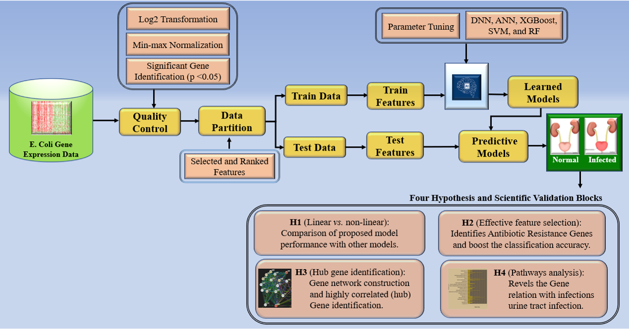 Fig. 3.
The overall architecture of aiGeneR and other studied models. XGBoost, eXtreme Gradient Boosting.
A large number of samples are needed to train a deep-learning model because a limited training set will result in overfitting. The accuracy curves and loss curves of the training and validation sets provide the most detailed insight into the fitting process. The training and validation set curve trends should be comparable to one another for optimal fit. A reduction in model complexity is required if the accuracy or loss of the training set differs from those of the validation set. These differences indicate overfitting. The performance of the model prediction needs to be enhanced in the absence of underfitting [52].
We construct a basic Multilayer Perceptron (MLP) neural network to perform a
binary classification job with prediction probability for DNN. The Keras library,
which is based on Tensorflow, is commonly used in Python 3.7 (Python software
foundation, Wilmington, DE, USA) [53]. The input dimension of the dataset is 30.
One hidden layer comes before one output layer. The accuracy score is the
measurement of the model performance. If there has been a significant rise in
accuracy (
The dataset for this work is obtained from the National Center for Biotechnology Information (NCBI) and the source (URL) of the dataset is “https://www.ncbi.nlm.nih.gov/geo/query/acc.cgi?acc=GSE98505”. The dataset explores the historical function of the synthetic protein MalE-LacZ72–47 in causing cellular stress and its deadly impact on bacteria. The study’s focus on downstream metabolic processes shows that the ROS-dependent component of antibiotic lethality and MalE-LacZ lethality are identical. Growing in M63 medium, E. coli MC4100 cells expressing a MalE-LacZ hybrid protein under a maltose promoter (MM18) were stimulated with 0.2% maltose. To extract RNA, the cells were shaken and incubated at 37 °C for five hours. Samples were taken every hour. Increased susceptibility is seen in oxidative stress-sensitive mutants, suggesting that reactive oxygen species (ROS) cause cell death. The number of samples and genes in this dataset are summarized in Table 1. However, it is found that the dataset taken for our experiment is balanced with both positive and negative samples. The raw data and the processed data are the same since no genes with null values greater than 30% were discovered during the imputation phase.
| Dataset Type | Genes | #Total | #Normal | #Diseased |
| Raw Data | 10208 | 36 | 18 | 18 |
| Processed data | 10208 | 36 | 18 | 18 |
| Dataset (with p-value |
5571 | 36 | 18 | 18 |
We found that the dataset (GSE98505) is having null values and the expression value ranges from 0 to 16. We aim to remove the genes which are having more than 30% null values but, there are no such genes identified. To reduce the computational burden, we apply the normalization process to the dataset. The data pre-processing phase includes data imputation, normalization of the raw data, Log2 transform, and p-value measure [14].
In the first step of data processing the duplicate values are removed. Some well-accepted imputation methods for numerical features includes rounded mean. In this case, the approach substitutes null values for that feature’s mean, rounded mean, or median values found across the whole dataset. The rounded mean data imputation technique is used to fill in the null or missing values. The method aids in maintaining the data’s overall distribution by substituting missing values with the rounded mean [54]. The rounded mean imputation technique keeps part of the variable’s statistical characteristics [55].
Data normalization is done in the second step of data preprocessing. Here we deploy the min-max normalization technique. The min-max normalization normalizes the data without disturbing the other data due to variance in their original scale and it reduces all features to a standard and single scale which is best fit for our dataset [56]. However, it is also found that many machine learning algorithms’ convergence rates and performance can be enhanced by normalizing features using min-max normalization [57].
The third step of the data processing includes the Log2 transformation. For gene
expression data, the Log2 transformation reduces the dynamic range, makes
interpreting fold changes easier, and improves statistical stability and
visualization. The fourth and final step of data processing holds the processed
data based on a p-value less than 0.05. R statistical software (version
4.2.0, The R Foundation for Statistical Computing,
https://www.r-project.org/foundation/) was used to perform all statistical
analyses [58]. With a statistical significance criterion of p
Artificial neural networks (ANNs) and deep neural networks (DNNs): Because they are capable of accurately capturing the intricate interactions between genes and phenotypes, ANNs and DNNs are frequently utilized in gene expression data processing. These models work especially well for tasks like predicting disease outcomes and classifying gene expression. As our work also focuses on gene network analysis, where the objective is to find interactions between genes, the performance of ANNs and DNNs is found significant [59, 60, 61]. The reason behind choosing ML models like XGBoost, SVM, and RF is, these models can handle high-dimension data, are robust to overfitting, and have the ability of non-linear transformation [24]. In addition to this, XGBoost can be utilized to predict the course of a disease or find biomarkers for particular illnesses (cancer) [18]. SVM is frequently employed in the study of gene expression data because it is capable of revealing intricate connections between genes and phenotypes. Similarly, RF is frequently utilized to predict the course of a disease or find biomarkers for particular diseases using gene expression data [62, 63].
In this study, the proposed aiGeneR is the capsule that binds the DNN algorithm for classification which performs incredibly well on the feature that the XGBoost model has selected. The model accuracy of aiGeneR improved significantly compared with the model run on raw data and the model run with selected features. The general equation for XGBoost feature selection is shown in Eqn. 1,
Where the predicted value of input data b is
The aiGeneR performs the classification problem by combining the XGBoost feature selection algorithm and DNN architecture. This paradigm gives the genes that are prone to antibiotic resistance, informative for disease prediction, and hub genes, which are in charge of tightly managing a large number of genes through strong cluster correlation. The biological validation section (section VII) explains in various points about this.
The following is the algorithm for XGBoost feature selection and DNN (aiGeneR) which gives the best classification result compared with other ML models.
Step 1: Divide the dataset into train test sets (7:3). Run the XGBoost model with all the features (Baseline model).
Step 2: Repeat each feature’s evaluation using XGBoost to determine its significance. Metrics like feature gain is used to evaluate a feature’s significance.
Step 3: Choose the Top-10, Top-20, and Top-30 features from the XGBoost feature ranking output.
Step 4: To create and train the DNN classifier, import the necessary libraries, such as TensorFlow or Keras.
Step 5: The Top-10, Top-20, and Top-30 features will be the input to the DNN model.
Step 6: Finally make the training and test sets on the input. The testing set will be utilized for evaluation, while the training set will be used to train the DNN classifier.
Algorithm 1 aiGeneR
##Taking the gene expression raw dataset as input
Input: Dataset DS (X = 36, Y = 10576): The set of samples and genes
## The quality control and feature ranking
Output: Normalized DS, p
Feature selection (X = 36, Y = 5730)
Feature Ranking [DS1(X = 36, Y = 10), DS2(X = 36,
Y = 20), DS3(X = 36, Y = 30)]
## Splitting the ranked features into to train-test set
Split the DS to DS
## Proposed DNN model implementation phase
FOR (ILR = 1
Weight {W
FOR (HLR = 1
FOR (W= W
FOR (WE
FOR (N
N
Wi* ILR
OP
………+
W
OP
………+
W
END
END
END
END
END
The DNN used in aiGeneR is intended to classify E. coli bacterium infection in biological samples. It consists of several artificial neural layers, with two hidden layers positioned in between the input and output layers. The network architecture is specifically designed to handle the input data with 27 features and generate accurate classification results.
Architecture:
(a) Input layer: There are 27 nodes in the input layer, each of which corresponds to a different attribute that was taken from the biological samples. These qualities include the expression value of different genes in the sample.
(b) Hidden Layer: This deep neural network has two hidden layers, each with 12 nodes. These hidden layers act as processing units in between, converting the incoming data into a feature space that is more abstract and representative. A rectified linear unit (ReLU) function serves as the activation function for each node in the hidden layers, which each apply a weighted sum of inputs from the layer before. This non-linearity makes it possible to identify intricate linkages in the data.
(c) Output layer: There is just one node in the output layer. The anticipated chance that the input sample is contaminated with E. coli is represented by the output node’s activation value in this binary classification problem. Typically, a sigmoid activation function is used to compress this number into the range [0, 1], with values closer to 1 denoting a higher likelihood of infection.
A labelled dataset of E. coli-infected and non-infected samples is utilized to train the DNN. Through the use of an optimization technique called Adam, the network learns to modify the weights and biases attached to each link between nodes in the layers. Utilizing a loss function that measures the discrepancy between expected and real labels, the network’s performance is assessed. Binary cross-entropy is a typical loss function for binary classification applications. To achieve optimum performance, hyperparameters like the learning rate are set at 0.0001 and batch size is 42. In order to prevent over fitting, a 3-fold cross-validation is also used during training. This deep neural network architecture in aiGeneR 1.0, which includes 27 input nodes and two hidden layers, was created especially for classifying E. coli infections in biological samples.
In the above algorithm, ILR contains the input layer nodes and HLR contains the
hidden layer nodes. W and WE
In this section, we discussed the working procedure of the DNN classification model. The deployment of the proposed model is done with the architectural modification of the baseline DNN model. We focus on the model evaluation techniques, evaluation metrics used, and baseline model of DNN for our work. The implemented DNN model has having input layer, two hidden layers, and one output layer. The DNN model was trained for 20 epochs, with 2 samples in each batch. To prevent overfitting, an early stopping mechanism was also implemented. The early halting mechanism, which reduced the learning rate to 0.001 of the previous learning rates, was activated specifically if the accuracy in the validation set did not increase by 0.0001 within 17 epochs. The Top-10, Top-20, and Top-30 features chosen by the XGBoost feature selection model is used to determine the number and dimensions of aiGeneR model’s input nodes.
Building an AI protocol for identifying the ARG using gene expression data is essential. Gene expression data are typically complicated and nonlinear in nature. It is crucial to comprehend how non-linear classifiers behave when applied to gene expression data. We believe that when using gene expression data, non-linear classifiers exceed linear approaches. Additionally, it is crucial to extract the most crucial features because they are crucial to classification performance [64, 65]. The selection of the classification model’s feature count is equally critical. To examine these two key points on linear vs. non-linear models and effective feature selection, we perform the below experiments;
(1) Experiment #1 (E1): Training the models and comparison of linear and non-linear ML models.
(2) Experiment #2 (E2): Effective features are selected by evaluating the feature selection model on the processed gene expression data.
The proposed aiGeneR model consists of four major steps namely quality control, effective feature selection, classification, and biological interpretation as shown in Fig. 3. The main functionality of this model is to extract significant features, observe the model performance, and reduce the computation burden. However, the computational time is much less if the learning model operates with selected features [66].
The different steps of this deployed model are, step-1 includes the used dataset, step-2 holds the data preprocessing and feature selection used for data preparation, and step-3 is meant for the classification of infected samples. The last section of our proposed model (step 4) represents the hub gene identification and biological validation. The basic operation of the model starts with the data pre-processing and feature selection process as used by our group previously [67]. Here we evaluate the XGBoost feature selection model to find the most significant features from the dataset. The evaluation is based on training the XGBoost model on our dataset using the labels as the target variable and the gene expression levels as features. According to how much each feature (gene) contributes to the prediction, XGBoost automatically gives importance scores for every feature (gene) during the training phase. The advantages of the XGBoost feature selection technique help to find significant features which helps to increase model accuracy. The ability of the XGBoost feature selection technique to deal with missing values, outliers, and non-linear data makes it more popular, which is shown in this section [68].
The open-source machine learning algorithm eXtreme Gradient Boosting (XGBoost) is made to handle issues with regression, classification, and ranking [64, 67]. It is a modified form of the gradient boosting technique that is frequently used in both commercial applications and data science competitions. Some of the important features of XGBoost are,
(a) Handling missing values: Internally, XGBoost can tackle missing values by discovering how to effectively fill in the gaps with the information that is currently available.
(b) Regularization: L1 and L2 regularization are used by XGBoost to reduce overfitting and increase the model’s generalizability.
(c) Feature importance: To comprehend the fundamental patterns in the data, XGBoost offers a way to quantify the significance of every feature in the model.
(d) Faster Processing: To make the model learn more quickly, XGBoost opted for parallel processing which utilizes several CPU cores.
The machine learning method XGBoost uses decision trees as its foundation. Regression, as well as classification problems, are addressed by it. A group of decision trees is assembled using XGBoost, and each tree learns from the mistakes of the one before it. After the learning process of each tree is completed, the forecasts of every tree in the ensemble are combined to get the final prediction [69].
There are two different categories of learning models used in this study: linear (Appendix A) and non-linear (Appendix B). We evaluate all of the models according to their performance in two categories: linear classification model performance and non-linear classification model performance. It is observed that non-linearity in the dataset affects the performance of the linear models, while the non-linear model performs remarkably well.
There are a total of five learning models deployed in this experiment out of which aiGeneR, ANN, and XGBoost are non-linear learning models, and SVM, RF are linear learning models. Three non-linear models’ mean accuracy is 88.33%, compared to two linear models mean accuracy of 67.50%. The non-linear learning model has a mean accuracy that is 22% higher than the linear models when we compare the top two performers from each learning model which satisfies our hypothesis. Similarly, the computational time taken by the non-linear model is less compared with the linear model. The comparison statistics in terms of classification accuracy and computational time of the linear and non-linear learning models are provided in Table 2.
| Model (Top-2 learning models from each group) | Mean Accuracy (%) | Mean Computational Time (Sec) | |
| System-1 | System-2 | ||
| Non-linear | 89.50 | 06.62 | 11.70 |
| Linear | 74.50 | 15.06 | 26.24 |
Features selection and optimization are crucial processes in the analysis of gene expression data. The selection of the most pertinent features becomes essential for correct insights and model performance because many genes may influence outcomes [24]. Finding a selection of genes that cause the observed changes is the goal of this technological study.
The genes are selected by deploying the XGBoost feature selection model. The top-ranked genes selected by the XGBoost model are then used by the different classifiers proposed in this work. The XGBoost feature selection model is implemented on the 5571 genes selected after data preprocessing. The XGBoost feature selection model selects and ranks 479 genes as shown in Fig. 4.
 Fig. 4.
The genes selected by the XGBoost feature selection model with their importance score and Gene number. XGBoost, eXtreme Gradient Boosting.
In Fig. 4, a few Top-ranked genes which are having feature importance scores of more than 0.01 are marked with different color (blue, orange, and dark green) than other selected genes. The highest feature importance score obtained is 0.24 and the lowest is 0.00014. We then take the Top-10, Top-20, and Top-30 ranked genes and form three different datasets, and applied the classification model to these datasets. The Top 30 genes based on their feature importance score are shown in Fig. 5.
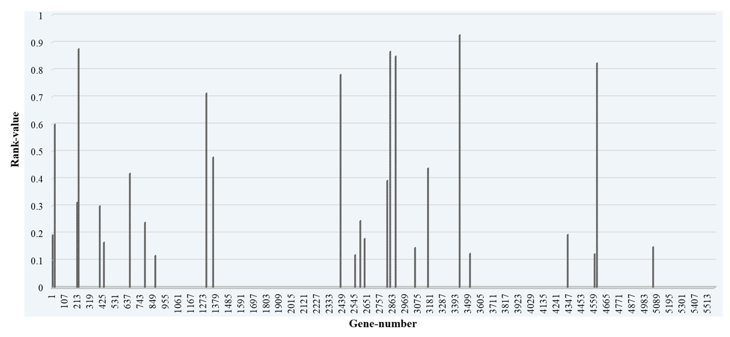 Fig. 5.
Top-30 ranked genes with their rank value and gene number.
Classification is just one of the many machine-learning tasks that can be performed with ANNs. An artificial neural network collects input data for a classification problem and outputs a categorical result. The classification performance of the learning model highly depends on the model tuning. Model tuning is a crucial phase in the ML process since it can enhance the model’s functionality and increase its predictive power [70]. A few key parameters for the deployed ML models in this work are discussed below.
The dataset we have taken has having small sample size, a short validation set would not give a reliable indication of the model’s performance. K-fold cross-validation is one way to handle such a situation [71, 72]. Except for the class distribution of the dataset being kept throughout the splits, the splitting technique is similar to the repeated K-fold cross-validation. In other words, each fold will have an identical distribution of samples across classes as the original dataset. So, for classification tasks with unbalanced class distributions, stratified K-fold cross-validation will be more appropriate [52, 72]. In our implementation phase, we take the k value as 3 for all the models. The deployed XGBoost, SVM, and RF classification model has followed the K-fold cross-validation from the train-test split. Based on the validation accuracy, precision, recall, f-score, false positive rate (FPR), and false negative rate (FNR), the XGBoost, SVM, and RF model performance is evaluated.
The deep network-based classification model used in this study was tested using the same methodology as the classification models mentioned in Section 4. Training and validation accuracy curves and loss curves were initially plotted to pre-screen experimental configurations with good performance to choose the best set of hyper-parameters for the model. The best parameter combination was then chosen by repeating the trial settings with good performance 3CV 10 times and using the average AUROC as an evaluation indicator. The performance of the ANN and DNN models is measured based on the validation accuracy (ACC), precision (PRE), sensitivity (SEN), specificity (SPE), f-score (F1), FPR, and FNR (Appendix C).
The anaconda environment and Jupiter notebook are utilized to perform the model architecture design and parameter setting. The learning models are implemented with Python (version 3.7) programming language [73, 74]. The results obtained using this proposed approach and a discussion along with the exploratory data analysis are presented in this section. The proposed model is developed on two different computational systems. The first system (system-1) is a workstation with 32 GB of Random Access Memory (RAM), 1 TB of SSD storage, an Intel Core i7 processor, and an Ubuntu 20.04 operating system. The specification of the second system (system-2) is 8GB of RAM, 256 SSD and 1 TB HDD, an Intel core i5 processor, and a Windows 10 operating system. The performance comparison of the implemented model in terms of computational time on these two systems is shown in Table 3.
| System-1 | System-2 | ||||
| AI Classifiers | Computational time in (sec) | Raw Data | Selected Features | Raw Data | Selected Features |
| SVM | 21.13 | 13.90 | 38.20 | 26.14 | |
| RF | 33.21 | 16.23 | 51.32 | 26.35 | |
| XGBoost | 25.90 | 11.30 | 42.31 | 19.52 | |
| ANN | 18.04 | 06.01 | 23.12 | 11.81 | |
| aiGeneR | 17.43 | 07.23 | 23.09 | 11.60 | |
SVM, support vector machines; RF, Random Forest; ANN, artificial neural network; AI, artificial intelligence.
The computational time taken with system-1 specification is much less than with system-2. It can also be observed from Table 2 that the classification models are taking very little time with the selected features as compared to the raw dataset. It is seen that the classification model like DNN, and ANN takes significantly less time with selected features for defined objectives in comparison to other considered classifiers. The average computational time for all the implemented models in the case of raw data as input is 23.14 sec and 35.60 sec for system-1 and system-2 respectively. The average computational time for all the implemented models in the case of the selected feature for the classification task is 10.93 sec and 18.88 sec for system-1 and system-2 respectively. Using selected features for the classification task led to a considerable reduction in computational time, with an average drop of 47.23% in system-1 and 53.03% in system-2 compared to the computational time required for raw data classification (without feature selection).
Our proposed model, aiGeneR, is quantified in this section, along with a thorough examination of its correctness. For its remarkable predictive abilities in a variety of tasks, from classification to regression, the aiGRNER 1.0 algorithm, a variation of the XGBoost method with the DNN classification algorithm, has drawn a lot of attention. Our goal is to thoroughly evaluate the accuracy of aiGeneR and learn more about its performance traits using various datasets.
The model metrics for different learning models with raw datasets (without feature selection) are shown in Table 4, and Fig. 6 shows the performance of these learning model metrics. With an impressive classification accuracy of 75%, the non-linear aiGeneR model outperforms the linear SVM. The measures show that the proposed aiGeneR model exceeds the other model in terms of classification accuracy which is more than 20% than XGB+ANN, XGB+XGB, and XGB+SVM classification models. It is observed that the XGB+RF classification model resulted in poor accuracy of only 37% and 0% specificity which indicates a large number of false positives and an inability to correctly detect negative examples.
| Raw Data (without feature selection) | |||||||
| The performance metrics are in percentage (%) | |||||||
| FS+Classifier | ACC | PRE | SPE | SEN | F1 | FPR | FNR |
| XGB+ANN | 62 | 50 | 60 | 66 | 57 | 40 | 33 |
| XGB+XGB | 62 | 75 | 66 | 60 | 66 | 33 | 40 |
| XGB+SVM | 62 | 50 | 60 | 66 | 57 | 40 | 33 |
| XGB+RF | 37 | 75 | 0 | 42 | 54 | 100 | 57 |
| aiGeneR | 75 | 75 | 75 | 75 | 75 | 25 | 25 |
ACC, accuracy; PRE, precision; SEN, sensitivity; SPE, specificity; F1, f-score; FPR, false positive rate; FNR, false negative rate; FS, feature selection.
 Fig. 6.
Classification model metrics for all the models on raw data.
Across three different feature sets, the aiGeneR model showed promise in classification tasks as shown in Table 5. The model produced relatively high accuracy and precision while maintaining a reasonable balance between recall and precision when tested using the Top-10 attributes. When the aiGeneR model was tested using the Top-20 features, its performance significantly improved. A stronger overall ability to predict and a more balanced trade-off between precision and recall are shown by improvements in accuracy, recall, and F1 score. The experiment is carried out based on the protocol discussed in the experimental protocol (EP) in section IV.
| ML Model | Accuracy | Precision | Recall | F1 | Specificity | FPR | FNR | |
| Top-10 | XGB+SVM | 57 | 57 | 66 | 57 | 57 | 0.37 | 0.37 |
| XGB+RF | 64 | 85 | 60 | 70 | 75 | 0.11 | 0.44 | |
| XGB+XGB | 64 | 71 | 62 | 66 | 66 | 0.22 | 0.33 | |
| XGB+ANN | 78 | 71 | 83 | 77 | 75 | 0.18 | 0.09 | |
| aiGeneR | 85 | 100 | 77 | 87 | 100 | 0.10 | 0.16 | |
| Top-20 | XGB+SVM | 78 | 71 | 83 | 76 | 75 | 0.25 | 0.16 |
| XGB+RF | 71 | 85 | 66 | 75 | 80 | 0.20 | 0.33 | |
| XGB+XGB | 86 | 87 | 87 | 87 | 83 | 0.12 | 0.16 | |
| XGB+ANN | 86 | 86 | 86 | 86 | 86 | 0.14 | 0.14 | |
| aiGeneR | 93 | 100 | 87 | 93 | 100 | 0.00 | 0.12 | |
| Top-30 | XGB+SVM | 78 | 71 | 83 | 76 | 75 | 0.25 | 0.16 |
| XGB+RF | 71 | 85 | 66 | 75 | 80 | 0.20 | 0.33 | |
| XGB+XGB | 86 | 87 | 87 | 87 | 83 | 0.12 | 0.16 | |
| XGB+ANN | 86 | 86 | 86 | 86 | 86 | 0.14 | 0.14 | |
| aiGeneR | 93 | 100 | 87 | 93 | 100 | 0.00 | 0.12 |
A stronger overall ability to predict and a more balanced trade-off between precision and recall are shown by improvements in accuracy, recall, and F1 score. The perfect specificity and low false positive rate demonstrate that the model has sustained superior performance in correctly classifying negative samples. However, for the Top-30 feature, the performance of aiGeneR is unchanged. The proposed aiGeneR (XGBoost feature selection and DNN classification) model successfully used feature information to generate precise predictions for the classification problem. It is crucial to note that the model’s performance was considerably impacted by the choice of the most significant features, highlighting the significance of feature engineering and selection in machine learning pipelines.
To choose the most insightful features from the dataset, we used three separate datasets based on feature selection (ranking). The datasets are Top-10, Top-20, and Top-30. The five different classification algorithms aiGeneR, ANN, XGB, SVM, and RF were also coupled with these features to create a comparative classification model. Performance measures like accuracy, precision, recall, F1 score, specificity, false positive rate, and false negative rate are taken into consideration for the deployed model’s potential testing on the identification of infected and non-infected samples. Figs. 7,8,9 show the model metrics on Top-10, Top-20, and Top-30 genes respectively, and Fig. 10 summarizes the performance of all these model metrics in terms of classification accuracy.
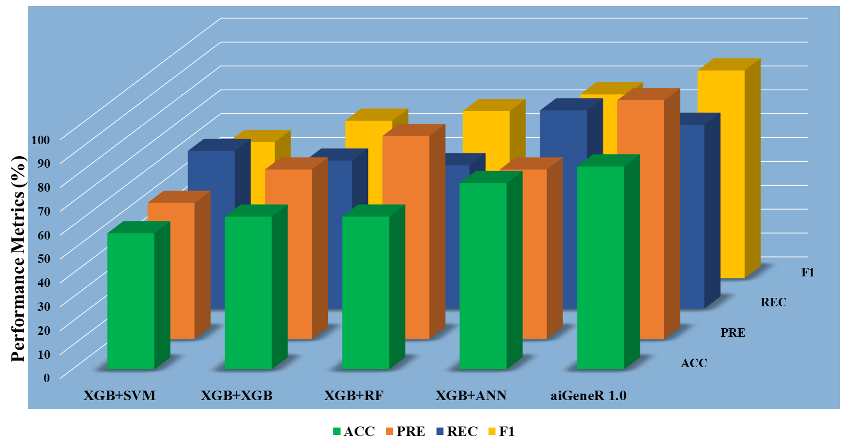 Fig. 7.
Classification metrics of all the models (Top-10 features).
 Fig. 8.
Classification metrics of all the models (Top-20 features).
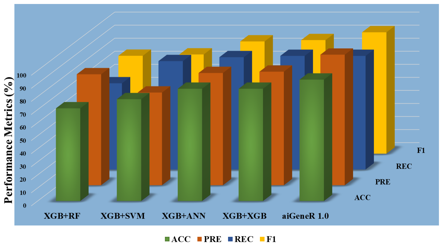 Fig. 9.
Classification metrics of all the models (Top-30 features).
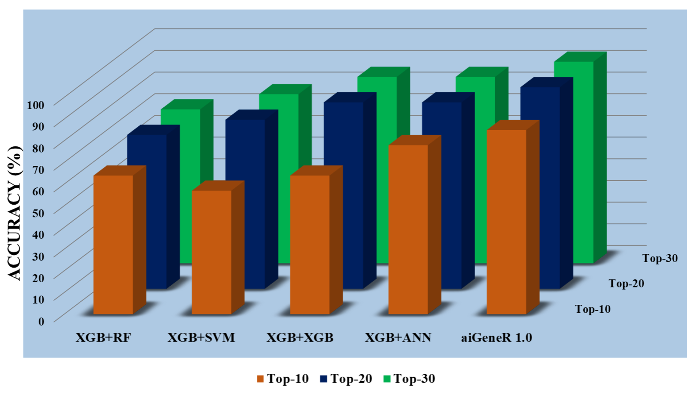 Fig. 10.
All Models accuracy on Top-10, Top-20, and Top-30 features.
Using XGBoost feature selection techniques, we compared how well machine learning models performed at classification tasks during the experiment phase. The outcomes revealed that the adoption of the feature selection technique significantly affects the model’s classification performance. When compared to how these models perform on raw data, it is also seen that classification models applied to the Top-20 features yield the best classification accuracy. Additionally, models with fewer features lighten the computational load and offer the best classification accuracy. In addition to this, high accuracy and precision were continuously attained by aiGeneR, making it an excellent contender for classification tasks for our defined objective. This observation is obtained with model evaluation metrics in experimental protocol (EP) section (section IV).
The observation in figure (Fig. 10) clearly shows that the aiGeneR model acquires a higher classification accuracy of a minimum of 10.08% (for all the 30 ranked feature datasets) and a maximum of 14.9% (for the Top-10 ranked feature dataset) in comparison to the other proposed models. However, it is also seen that all the proposed models perform well on the selected feature set of Top-20 and Top-30 as compared with the Top-10 feature set (Appendix Table 11). It can be concluded from our hypothesis that; the proper selection of significant features boosts the performance of the classification model in terms of accuracy. A minimum of 20 features is needed by aiGeneR to attain the best model accuracy.
The false positive rate (FPR) and false negative rate (FNR) for all the implemented models on the Top-ranked feature dataset are shown in Fig. 11. The minimum FNR and FPR for each feature set is denoted as A1, A2, A3 and B1, B2, B3 respectively. The FPR and FNR values are the same for SVM in Top-10 features set is denoted by C1 and for ANN model on Top-20, and Top-30 feature set is denoted by C2 and C3. The average FPR for the Top-10, Top-20, and Top-30 feature datasets is 0.98, 0.52, 0.74 and the average FNR is 1.39, 0.72, and 0.69 respectively. It is observed that the FPR and FNR are reduced with Top-20 and Top-30 ranked features (genes) as compared to Top-10 ranked features.
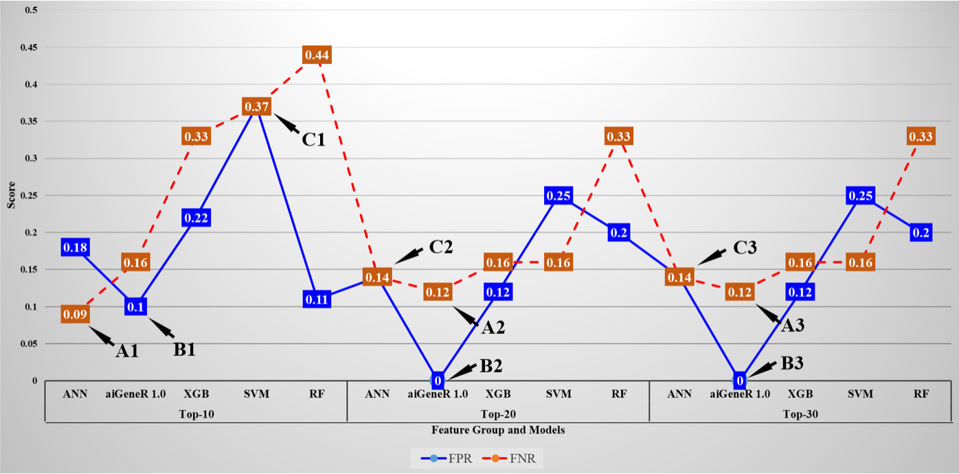 Fig. 11.
False positive rate and False negative rate of all the studied models for Top-10, Top-20, and Top-30 ranked features.
The XGBoost feature selection algorithm applied to the raw data selects 471 (four hundred seventy-one) initial features as shown in Fig. 4. The selection is based on feature ranking which uses the Gini index for ranking the selected genes and can be visualize in Fig. 5. In this work, we take the Top-30 ranked genes for the analysis of the performance of the proposed models. We carefully searched for the presence of the AMR genes in the dataset, and it was found that there is a single AMR gene present in the dataset, and that gene is selected and ranked among the Top-30 genes by the XGBoost model. The selected Top-30 ranked genes and their feature importance number (the position of genes in the dataset), and gene symbol are shown in Table 6 and the characteristics of these (aiGener-identified) genes are shown in Appendix Table 12 (Ref. [57, 58, 59, 60, 61, 62, 67, 68, 69, 70]) (Appendix F).
| Rank | F# | Gene ID | Gene Symbol | Rank | F# | Gene ID | Gene Symbol |
| 1 | 3512 | 1765606 | paal | 16 | 4333 | 1767117 | NF |
| 2 | 2590 | 1763875 | NF | 17 | 1353 | 1761578 | ycgE |
| 3 | 400 | 1759806 | trpC // ECs1834 | 18 | 4 | 1759074 | yfbN |
| 4 | 210 | 1759472 | sepQ // ECs4565 | 19 | 867 | 1760673 | yfeR // ECs3281 |
| 5 | 2546 | 1763807 | ycfT // ECs1493 | 20 | 653 | 1760272 | uxuB // ECs5282 |
| 6 | 1296 | 1761463 | C2193 // ECs2497 | 21 | 22 | 1759103 | NF |
| 7 | 2841 | 1764345 | c0272 | 22 | 2887 | 1764429 | trpB // ECs1833 |
| 8 | 2626 | 1763963 | polB | 23 | 4579 | 1767567 | ECs2954 // Z3089 |
| 9 | 5051 | 1768435 | pspB | 24 | 4559 | 1767527 | rbn // yihY |
| 10 | 3050 | 1764734 | ECs3616 // Z4071 | 25 | 222 | 1759495 | NF |
| 11 | 2424 | 1763555 | ECs1418 | 26 | 435 | 1759866 | potF // ECs0934 |
| 12 | 780 | 1760513 | NF | 27 | 2683 | 1764051 | ECs2895 ///gatC |
| 13 | 2816 | 1764302 | ECs1074 // Z1338 | 28 | 1930 | 1762651 | adk |
| 14 | 3425 | 1765444 | NF | 29 | 991 | 1760885 | ECs4986 |
| 15 | 5664 | 1764672 | tetM | 30 | 790 | 1759741 | paaZ |
In addition to the above, the Top-30 ranked genes selected by the XGBoost feature selection model with their rank, feature importance number (F#), gene id, and gene name (gene symbol). This gene ranking table presents a prioritized list of the genes in the dataset based on their feature importance ratings. The genes that are ranked 1, 3, 8, 9, 22, 28, and 30 are highly correlated with other genes based on the number of genes connected to them.
Escherichia coli (E. coli) often carries the tetM gene. Tetracycline, a popular antibiotic used to treat various genes (gene-id) there are only 15 genes which are having their gene symbols. The tetracycline resistance genes are a family of genes that includes the tetM gene. ‘tetM’, a ribosome protection protein, is a protein that is produced by the tetM gene. It works by attaching to the ribosome and blocking the antibiotic tetracycline from attaching to the ribosomal target site [75]. The tetM gene is identified by our proposed model and ranked in 15th place as shown in Table 6. Due to the limited gene expression data availability for E. coli, the presence of ARG is very less. In this work, we deployed XGBoost feature selection method for its simplicity and significant performance over gene expression data. Several feature selection methods like PCA, LDA, t-SNE, PCA Polling can be tested on this data and comparison of classification performance may include in future work.
Building trustworthy and efficient predictive models requires an accurate assessment of model performance, which is a vital component. The capacity to evaluate a model’s performance serves as a crucial sign of its potential to address real-world problems in a variety of domains, from machine learning to scientific research [76]. This section examines a thorough assessment of our suggested models, considering several factors to provide readers with a solid knowledge of their abilities and shortcomings.
To assess the effectiveness of the model in various scenarios, we investigate several important factors. A comprehensive understanding of the model’s effectiveness is provided by each subsection, which is created to investigate a particular aspect of performance.
The Receiver Operating Characteristic (ROC) curve is a crucial indicator of a
classification model’s efficacy. We examine the performance analysis of our
proposed aiGeneR along with ANN, XGBoost, SVM, and RF with a value of
p
More importantly, the feature selection technique which provides the most significant features helps to improve the performance of the aiGeneR model. Fig. 12 shows the ROC performance of the five classification models (aiGeneR, ANN, XGBoost, SVM, and RF). Our proposed model aiGeneR has accomplished a remarkable milestone with a robust area under the curve (AUC) value of 98.4%. However, the ROC value of RF is lowest compared with all other classification models. In the analysis process of gene expression data despite the challenges of the implemented complex non-linear dataset aiGeneR achieves the best AUC value.
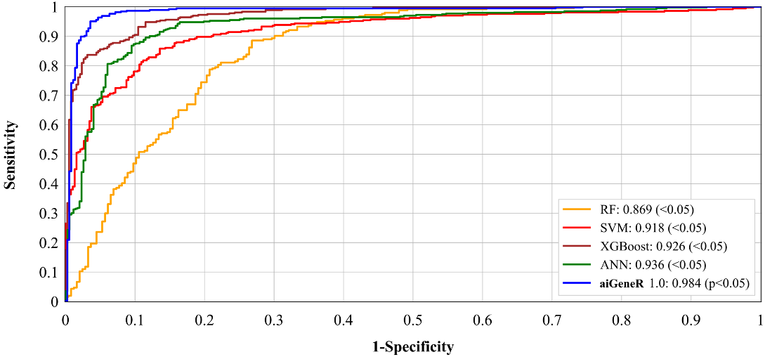 Fig. 12.
Receiver operating characteristic of all the classification models.
This study also comprehended the implemented model’s performance on all possible train-test split and the comparison of classification accuracy on test data. The size of training data has an impact on the learning model and makes the model generalized well to unseen data [34]. We evaluate our proposed model aiGeneR along with four other classifiers used in this study on a used dataset with different train-test splits. It is observed that aiGeneR requires very minimal cases for generalization whereas other models require a greater number of cases. The detailed discussion on the effect of data size on our proposed model is discussed in this section. All the possible train-test splits on the used dataset and the comparison of classification accuracy on test data are shown in Fig. 13.
 Fig. 13.
Visualization of classification accuracy achieved in different train-test splits of all the studied learning models.
The goal is to track how the train-test split ratio influences the performance of the model as per the EP (section IV) effect of data size. In the case of the aiGeneR classification model, as the percentage of training data rises, accuracy progressively rises. When using a 70:30 train-to-test split ratio, the model obtains the best accuracy of 93%. The XGBoost-based ANN, XGBoost, and SVM classification model achieves the best classification accuracy with the 70:30 train-test split and the RF classification model reaches the maximum accuracy with a 60:40 train-test split. Our observation on this analysis concludes, that all the studied learning model archives an optimum accuracy with a 70:30 train-test split.
Model generalization is the capacity of the model to function effectively on novel, untested data, suggesting its resilience and applicability for practical applications. The least number of unseen instances and minimum amount of data needed for the generalization of the proposed learning models are shown in Table 7. The least number of new instances and the minimum amount of data needed for model generalization are shown in the table for each machine learning model. We evaluate the model generalization on the Top-30 selected features with 36 samples (cases). A minimum of 40 data points is needed for generalization in both DNN and ANN models. Additionally, to validate the model’s performance on fresh data, at least 16 previously unreported cases are required. To achieve generalization, the XGBoost model needs a larger dataset with at least 70 data points and minimum of 25 instances is required for verifying unrecognized circumstances. Similarly, to achieve generalization, SVM and DT require 60 data points with 22 unseen instances.
| Model | Minimum (%) of Samples for Model Generalization | Minimum Unseen Cases |
| SVM | 70 | 25 |
| RF | 60 | 22 |
| XGBoost | 70 | 25 |
| ANN | 40 | 16 |
| aiGeneR | 40 | 16 |
We executed a power analysis to establish the minimal sample size required for precisely and accurately calculating a population proportion. The tests were carried out using the technique mentioned in [65, 77, 78]. The sample size calculation formula, denoted by the symbol Sn, is as follows,
Here, MoE stands for the margin of error,
As can be observed from Appendix Fig. 18 (Appendix D), the study has a sample size of more than what is necessary to meet the desired level of statistical power and classify accurately. The minimal sample size for the used dataset is also less than the amount of data accessible. However, to increase the classification model’s accuracy, statistical power, and precision, data augmentation may be used.
The process of confirming that a model or system satisfies its intended requirements is known as validation. Any model or system must go through this crucial stage in the development process, but it is especially crucial for models that will be utilized in high-stakes scenarios. We evaluate our proposed approach in a two-step validation, in step-1 we go for scientific validation, and in step-2 we do the biological validation. In scientific validation we evaluate the performance of the aiGeneR model to unseen gene expression data and in biological validation we do annotation of the outcome of our model.
The scientific validation of our proposed work uses the “Microarray transcriptomic profiling of patients with sepsis due to faecal peritonitis and pneumonia to identify shared and distinct aspects of the transcriptomic response” (E-MAT-5274) dataset which is available in ArrayExpress [73]. The characteristics of the dataset are described in Table 8. We evaluate our proposed model with the E-MAT-5274 dataset keeping all the model configurations and parameters as per our proposed pipeline. It can be observed from Table 9 that, the trend in the Top-20 and Top-30 selected feature groups achieves the same level of classification accuracy as our proposed model with the E. coli dataset.
| Data Type | Genes | Normal Samples | Diseased Samples |
| Raw Data | 47324 | 54 | 54 |
| Processed Data | 27160 | 53 | 53 |
| Dataset after applying a p-value less than 0.05 | 5000 | 53 | 53 |
| Model | Accuracy | ||
| Top-10 | Top-20 | Top-30 | |
| SVM | 57 | 68 | 77 |
| RF | 66 | 74 | 76 |
| XGBoost | 68 | 83 | 83 |
| ANN | 74 | 83 | 84 |
| aiGeneR | 81 | 91 | 91 |
This experiment indicated our proposed model may be used as a benchmark model for infected sample classification and informative gene identification using the gene expression datasets. The accuracy of classification achieved by aiGeneR on this dataset is still the greatest and has not altered, demonstrating the potential for the generalization of our approach. This indicates the validity of our claim that aiGeneR is a generalized model that can access various gene expression datasets to identify the most important genes.
This section explores the critical function of functional association and gene network analysis in biological validation. By highlighting the potential roles of important genes in particular pathways and processes and revealing coordinated patterns of gene expression, these approaches make it easier to evaluate high-dimensional gene expression data. The key to demonstrating the applicability and precision of these analytical methods is the coupling of computational predictions with experimental confirmation.
A database of observed and anticipated protein-protein interactions is called STRING. Protein-protein interaction networks are mathematical representations of the physical contacts between proteins in the cell [80]. The interactions come from computational prediction, knowledge transfer across species, and interactions gathered from other (primary) databases; they comprise direct (physical) and indirect (functional) correlations. This analysis section provides some summary network information, including the number of nodes and edges. The average node degree is the average number of interactions a protein has in the network. Higher numbers of edges reflect a dense gene cluster and a gene having maximum numbers of edges will be treated as the hub gene. Gene-network study provides a clear view of the identification of significant genes and pathways, discovers the functional association, prediction of gene function, and identification of hub genes. Disease biomarker and drug target identification is also the key contribution of gene-network analysis [81, 82].
The proposed learning model is tested on the Top-30 (thirty) ranked genes and found there are only 24 (twenty-four) gene names (gene symbol) available in the used dataset. Using these 24 genes the gene network is being constructed with the help of STRING and it is found that out of 24 genes, 15 genes are available in the STRING dataset. While comparing the Top-30 and Top-20 feature datasets we found that out of these 15 genes present in the STRING dataset, 11 are also present in the Top-20 feature dataset.
The strain used by our suggested model for the genes chosen is Escherichia coli K12 MG1655. We increase the number of genes in our experiment to build networks which will make it easier to comprehend how genes interact with one another. We, therefore, take into account an additional 60 genes that belong to the same strain as our observed genes (model-predicted genes). Finally, the gene network we tested included 75 genes from the K12 MG1655 strain out of which 15 genes are identified by our suggested model.
We searched for the connections and functional associations between our researched gene sets and other genes in E. coli to further confirm the filtered gene set. Utilizing the stringApp of Cytoscape [83], which maps the genes to the STRING database of interacting proteins [80], identified 15 significant genes (colored red), and 60 other genes were linked to the protein-protein interaction (PPI) network as shown in Fig. 14. STRING involves functional relationships from selected pathways, computational text mining, and prediction techniques as well as tangible connections from experimental data [84].
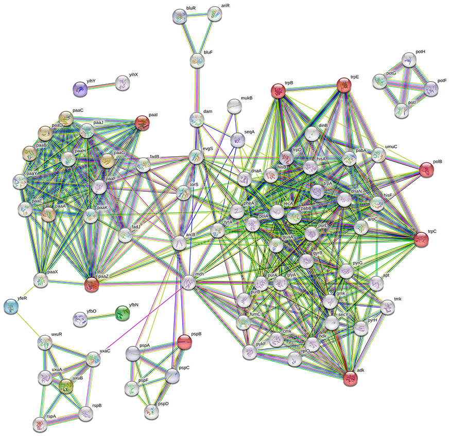 Fig. 14.
Gene correlation network of Top-30 ranked genes from aiGeneR with 60 other genes in the K12 MG1655 strain of E. coli.
The number of nodes is the same as the number of genes (75) and the expected edges is 156 but, the network constructed in STRING shows the number of edges is 360 which is a sign that the obtained genes create a significantly more interacting network than excepted. The Genes identified by our model (Top-30 gene group), especially paaZ, polB, trpC, trpB, adk, paaX, and trpE shows the maximum number of connected genes and gene cluster to them as shown in Table 6. The genes selected by aiGeneR are given additional properties to serve as hub genes according to the interaction edge we discovered in our gene network and the deep connections among the genes. The tetM an ARG identified by our proposed model is resistant to tetracycline. Both Gram-positive and Gram-negative bacteria can exhibit tetracycline resistance, which is mediated by the genes tetM and other related genes. Through horizontal gene transfer processes like conjugation, transformation, and transduction, this resistance can spread between bacteria [85]. The higher classification performance of aiGeneR with gene network analysis gives us a thorough understanding of the hub genes and the most important genes present in the dataset.
The bar graph in Fig. 15 depicts the findings of a pathway analysis, which revealed significant metabolic processes active in E. coli. Among the identified pathways, the cellular aromatic compound metabolic process, organic cyclic compound metabolic process, and small molecule metabolic process are especially important. These findings are consistent with previous E. coli research that has demonstrated the importance of these pathways in the bacterium’s metabolism [86, 87].
 Fig. 15.
Pathways association of selected Top-30 genes.
The analysis report also includes a few genes like PAAZ, PAAI, YFER, and UXUB that are connected to multiple pathways. These genes carry out novel metabolic processes in E. coli, including the hydrolysis of phenylacetyl-CoA and other aromatic molecules [88], which may be essential for E. coli to adapt to diverse environmental circumstances and use various carbon sources. However, certain genes listed in the table, such as POLB and ADK, have well-established roles in DNA replication, repair, and nucleotide metabolism, respectively. TRPB and TRPC, which encode enzymes involved in trypTophan biosynthesis, are also members of the well-studied trp operon in E. coli.
While these genes may not be associated with any new pathways, their presence in multiple pathways highlights their importance in E. coli metabolic processes. These findings provide a comprehensive overview of the metabolic network of E. coli and shed light on the interconnectedness of various pathways and the roles of specific genes within them. Further research into the functional significance of these pathways and genes will help us understand the physiology of E. coli and advance our understanding of microbial metabolism.
These pathways and genes selected by aiGeneR may also have implications for the pathogenesis of E. coli-caused urinary tract infections (UTIs), which are the most common cause of UTIs in humans. Some E. coli metabolism pathways and genes, such as those involved in iron acquisition, adhesion, toxin production, or biofilm formation, may contribute to virulence and survival in the urinary tract environment [89]. The genes identified by aiGeneR and the pathway analysis provide a detailed understanding of how these pathways and genes affect E. coli’s ability to cause UTIs could lead to new prevention and treatment strategies, especially in light of rising antibiotic resistance [89].
The genes displaying significant expression differences between the sick and
healthy samples were found using DE analysis. To detect the Differentially
Expressed Genes (DEGs), filtering criteria of padj(FDR) less than 0.05
(p
 Fig. 16.
The differentially expressed genes in the dataset after quality
control (with p-value
According to the findings, aiGeneR model (XGBoost feature selection and DNN) can be used as a standard model for significant gene selection and AMR gene identification, it also has certain limitations because of differences in the sizes and methods of the datasets that were taken into account. There is no information in the dataset used in this study regarding how the resistance developed about the sample preparation time. In section VI (B) we construct the gene network, the genes that are in the Top 30 are taken into consideration for network construction. It is observed from the constructed gene network that, the genes selected by the XGBoost feature selection model have AMR genes and are highly correlated with different gene clusters that may be affected by the resistance transferred by the identified ARGs. Therefore, we may draw a conclusion that the selected genes (Top-30) by our proposed model have significant analysis results on AMR gene identification and finding the genes that highly correlated with the maximum number of genes. During this work, we also found some important research information on AMR analysis and ARG identification which are listed below,
The performance of learning models in terms of accuracy is highly increased with Top-ranked datasets built on the features selected by the XGBoost feature selection model. The computational time for ML and Deep network models is significantly less while performing classification on Top-20 and Top-30 ranked feature datasets. The architecture of the implemented aiGeneR model is simple and able to provide high classification accuracy. The ARGs present in the dataset are identified and correctly classified with the aiGeneR model. The proposed aiGeneR (XGBoost + DNN) provides more accurate features and classification of infected and non-infected samples classification. The gene network construction gives a piece of detailed information on the genes that are selected by our model and their associatedness with other genes in terms of correlation factors. Our model identifies genes like Paaz, polB, trpC, trpB, adk, paaX, and trpEshown highly correlated with other genes and gene clusters. The chosen features are shown to be biologically significant and help the proposed model achieve a good level of prediction accuracy.
The core of our study involved applying hybrid ML models to classify E. coli infection cases and identify the relevant antibiotic resistance genes (ARGs). Deep network models were combined to create these machine-learning models. Therefore, it’s critical to compare our approach to earlier AI models. Considering this, we decided to compare our suggested models with earlier ML models (in AMR and other disease analyses) to directly address the benchmarking efforts.
There is an absence of research that combines ML and gene expression data to identify ARGs. Gene sequence information is used in the majority of research to classify resistance. Here, we evaluated two distinct gene expression and sequencing datasets that were utilized for cancer classification and AMR analysis in our benchmarking section. We chose cancer as the subject of our model benchmarking because machine learning has been used in numerous studies that use gene expression data.
For an accurate AMR analysis, data pre-processing, including cleaning, normalizing, and feature engineering, is essential. Several techniques in aiGeneR quality control pipeline, including min-max normalization, Log2 transform, a p-value criterion of less than 0.05, XGBoost feature selection, and deep neural networks, were used to find significant genes. Metrics like accuracy, precision, recall, and F1 score were used to assess the classification model’s performance on infected E. coli samples. The model achieved an F1 score of 93%, accuracy of 93%, precision of 100%, and recall of 87%. Additionally, the model’s adaptability to changes in the input data, generalizability to new data, and congruence with biological observations were all assessed. It is found that the model is reliable, generalizable, and consistent, according to the findings of these assessments.
Using gene expression data, our proposed aiGeneR model delivers hub genes and ARGs. The maximum classification accuracy is attained by the innovative, non-linear aiGeneR. Furthermore, the efficient feature selection used in our suggested pipeline plays a crucial role in improving classification accuracy. With various gene expression datasets, our suggested aiGeneR has demonstrated its generalizability while maintaining a high level of classification accuracy. The classification performance is enhanced by the significant genes that are identified by aiGeneR. It has also been noted that our approach achieves the maximum classification accuracy with just 20 genes. One of the most crucial features of our aiGeneR pipeline is its capacity to recognize hub genes, and the network analysis of the aiGeneR chosen has already demonstrated this assertion. Additionally, we assert that the aiGeneR identified genes are strongly linked to UTI, as revealed by the pathway analysis of these genes.
Four different models, including RF, DNN, DT, and srst2 [90], are implemented in [91]. The performance of DT was found to have a high classification accuracy of 91% when the models were evaluated based on classification accuracy. In this work, gradient boosting tree classifier is implemented with 0.1 learning rate, 300, 600, and 5000 boosting stages, deviance loss, and an 8:2 train-to-test split. Similar genetic characteristics that cause AMR are found in [92] by employing the SVM. Two SVM ensembles were created for each antibiotic case using the same feature matrix and AMR phenotypes: one with 500 SVMs trained on 80% of genomes with all features, and another with 500 SVMs trained on 80% of genomes with 50% of features, aiming to enhance SVM accuracy with high-dimensional biological data. It has been shown that the SVM model’s gene identification accuracy was 90%. However, most models that employ gene expression data choose feature selection techniques. The research published in [18, 30], and [93] used a variety of ML models to identify genes and categorize cancers. SVM, XGBoost, Neural networks, RF, and DT are the ML models used in this work. The XGBoost model in [18] achieves the best classification accuracy of 96.38%, the XGBoost model in [93] achieves the highest classification accuracy of 80%, and the SVM model in [30] achieves the highest classification accuracy of 96.38%. All these ML models are implemented on gene expression data. The work considered for this is shown in (Table 10, Ref. [18, 30, 91, 92, 93, 94, 95, 96]). A DeepPurpose DL model, which makes use of gene expression data, was deployed in [94] for the detection of Target genes and drug-resistant melanoma. The affinity score provided by the Deep Purpose (which is calculated based on the targeted genes and their potential drugs) is used as the performance measure. The model metrics are not provided in the publication; instead, the authors simply provide the number of genes that the model has identified. In [95], an experiment was conducted to predict antibiotic resistance using SVM and gene expression data. The model accuracy that was attained was 86%. Drug resistance and biomarkers in colon cancer identification are conducted by [96]. It obtains an AUC value of 0.6590 using gene expression data and elastic net regression.
| Year | Reference | Objective | AI Type | Method | Dataset | Performance Evaluation Metrics | Score (%) | Limitations |
| 2018 | Moradigaravand et al. [91] | Antibiotic resistance prediction | ML | GradientBoostingClassifier with a train-test split of 8:2, a learning rate of 0.1, with boosting stages of 300, 600, and 5000. | Whole genome sequencing. | Accuracy | 91 | The resistance detection mechanism of the model is unknown, and the model is not robust. |
| 2018 | Tian et al. [30] | Gene Selection and Classification | ML | Random forests, support vector machines (SVMs) with an RBF kernel, polynomial kernel SVMs, logistic regression, naive Bayes classifiers, and decision tree classifiers were used in 10-fold cross-validation on the discretized training data. | Phenotype gene expression data from mouse knockout experiments. | Accuracy | 80 | Feature combinations were not explored, and their influence on classification accuracy remains unstudied in the ML model’s performance assessment. |
| 2020 | Hyun et al. [92] | Genetic features that drive the AMR | ML | Use the same core allele/non-core gene encoding of genomes and the SVM-RSE technique to find AMR genes in the bigger P. aeruginosa and E. coli pan-genomes. | Genome sequence of 288 Staphylococcus aureus, 456 Pseudomonas aeruginosa, and 1588 Escherichia coli. | Accuracy | 90 | A substantial volume of data is necessary to assess the prediction accuracy of the models. |
| 2022 | Deng et al. [18] | Gene Selection and Classification | ML | The XGBoost-MOGA method combines the embedded XGBoost method with the wrapper MOGA method. | Cancer gene expression. | Accuracy | 96.38 | If there are more genes, the process of computing requires more. |
| 2023 | Cava et al. [93] | Cancer Classification | ML | Neural network with two hidden layers and each network node implemented the rectified linear unit (ReLU) as an activation function. RF with 500 numbers trees and XGBoost with a number of estimators 100. | Cancer gene expression. | Accuracy | 90 | Quality control, significant gene identification, and model generalization are missing. |
| 2022 | Liu et al. [94] | Target gene and drug-resistance melanoma identification | DL | Using Cytoscape and the STRING database, the PPI network was created. The survival analysis was carried out using GEPIA. DeepPurpose a pre-trained DL model is used to estimate the affinity score (drug-target interactions). | Melanomas (type of skin cancer) gene expression. | Affinity scores | – | Web-based tools are used for gene identification and biological validation of the results is missing. |
| 2006 | Györffy et al. [95] | Antibiotic resistance prediction | ML | SVM | 30 human cancer cell lines gene expression. | Accuracy | 86 | Expression analyses are not directly helpful for identifying potential novel variables functionally implicated in drug resistance. |
| 2022 | Li et al. [96] | Biomarkers in colon adenocarcinoma drug resistance | ML | Multivariate Cox analysis with elastic net regression and 10-fold cross-validation. | Gene expression derived from RNAseq. | Area-under-the-curve (AUC) | 65.90 | This work does not include any experimental validation of the proposed model or pathway analysis of the hub gene. |
It is not feasible to perform benchmarking specifically on ARG identification and classification of infected E. coli samples using gene expression data. As a result, we choose to compare our suggested model with the work in oncology. The model we propose is concentrated on E. coli infectious sample classification and ARG identification. The classification accuracy of the proposed aiGeneR is 93% with an AUC value of 98.4%, which is the highest of any model currently in use for AMR analysis of gene expression data. The generalizability of our model may be demonstrated by the classification accuracy and AUC of aiGeneR and its validation on the E-MAT-5274 gene expression dataset (section VII).
Access to diverse and extensive datasets that contain details on infections, drugs, and resistance mechanisms is necessary for AMR studies. Due to the restricted availability of such data, obtaining it might be difficult, particularly for rare or newly discovered resistance patterns. AMR data is intrinsically complex since it takes into account several variables, including bacterial strains, and environmental circumstances. It is a big problem to integrate and analyze these complicated datasets.
For an accurate AMR analysis, data pre-processing, including cleaning, normalizing, and feature engineering, is essential. Several techniques in the aiGeneR quality control pipeline, including min-max normalization, Log2 transform, a p-value criterion of less than 0.05, XGBoost feature selection, and deep neural networks, were used to find significant genes. Metrics like accuracy, precision, recall, and F1 score were used to assess the classification model’s performance on infected E. coli samples. The model achieved an F1 score of 93%, accuracy of 93%, precision of 100%, recall of 87%, and. Additionally, the model’s adaptability to changes in the input data, generalizability to new data, and congruence with biological observations were all assessed. It is found that the model is reliable, generalizable, and consistent, according to the findings of these assessments.
The aiGeneR learning model revealed that the genes paaI, trpC, polB, pspB, trpB, adk, paaZ, and tetM were significant. Expertise in microbiology, genetics, bioinformatics, and machine learning is frequently needed for effective AMR investigation. To address the complexities of AMR, multidisciplinary collaboration is required.
The application of ML models and neural networks for ARG detection and classification is the primary concern of this work. The work demonstrates a significant improvement in the identification of informative genes, the discovery of ARGs, and the classification of non-linear gene expression data sources, making the suggested aiGeneR a benchmark in the field of ARG identification. In comparison to previous studies on gene expression datasets for ARG detection, the aiGeneR model performs remarkably well. Additionally, the system’s robustness and domain adaptability are demonstrated by cross-validation, biological validation, and unseen implementations, as well as through how effectively it operates in domains other than the specific one on which it was trained.
This pilot study concerning the discovery of ARGs using gene expression data is highly motivated. This study can be expanded upon with data augmentation, perhaps leading to improved model performance. However, physicians do not recommend this strategy (the augmentation of medical data) because it is medically erroneous [97, 98]. If the model has been trained using synthetic data, we may get better model metrics. There are a few biases in our model that could be eliminated with more research, including (i) a smaller number of studies, (ii) the use of data augmentation, (iii) comparisons with other ML and DL models, (iv) no comments on the clinical validation, and (v) a description of benchmarking studies [99, 100, 101, 102, 103, 104].
Future work on enhancing ARG identification will focus on creating fresh datasets and investigating cutting-edge architectural concepts like Synthetic Minority Over-sampling Technique (SMOTE). We aim to assess the performance of these new models and conduct a variability analysis by contrasting them to our current aiGeneR models, such as the combination of ML with exhaustive feature space with DL.
Additionally, to improve the performance of the classification model, we intend to create a new quality control pipeline for the non-linear gene data. We want to work on analyzing research and ranking them according to their bias. Design systems can also be pruned to lower the size of the training models, and artificial intelligence designs are subject to bias.
Antibiotic resistance genes (ARGs) were identified and infectious and non-infectious samples were classified using a hybrid gene selection and classification approach using aiGeneR and XGBoost-based classifiers (ANN, SVM, XGBoost, and RF). As opposed to using the raw dataset, the results demonstrated that XGBoost feature selection significantly enhanced classifier performance. The aiGeneR model identified the tetM gene as an ARG responsible for decreased antibiotic efficiency through horizontal gene transfer, with the greatest classification accuracy of 93% with Top-20 and Top-30 ranking features. Whole Genome Sequencing (WGS) is used for AMR investigation and produces biologically significant data, although it is expensive. The discovery of AMR genes is complicated by a scarcity of gene expression data. AMR pattern and gene identification are made easier by WGS, notwithstanding the complexity of its processing. Future studies will use synthetic gene expression data from E. coli and deep learning models to overcome the limits of gene expression data to increase classification accuracy in AMR research and use WGS for ARG discovery, particularly in E. coli.
AI, Artificial Intelligence; AMR, Antimicrobial Resistance; ARG, Antibiotic Resistance Genes; ANN, Artificial Neural Network; DEG, Differentially Expressed Genes; DNA, Deoxyribonucleic Acid; DNN, Deep Neural Network; DL, Deep Learning; DT, Decision Tree; EP, Experimental Protocol; GA, Genetic Algorithm; IEEE, Institute of Electrical and Electronics Engineers; KNN, K-Nearest Neighbor; ML, Machine Learning; NN, Neural Network; RAM, Random Access Memory; RBF, Radial Bias Function; ReLU, Rectified Linear Unit; RF, Random Forest; SVM, Support Vector Machine; UTI, Urine Tract Infection; WGS, Whole Genome Sequencing; XGBoost, eXtreme Gradient Boosting.
The dataset used in this study is freely available in NCBI with accession no.: GSE98505.
DSKN, JSS, and TS: Study conception and design, data collection, analysis and interpretation of results, and manuscript preparation. DSKN, SM, SPR, SS, and SKS: Collect the data, perform the biological validation of the results, and manuscript preparation. DSKN, MMF, NS, ERI, and LS: Annotating the results and perform the biological validation of the results. All authors contributed to editorial changes in the manuscript. All authors read and approved the final manuscript. All authors have participated sufficiently in the work and agreed to be accountable for all aspects of the work.
Not applicable.
Not applicable.
This research received no external funding.
The authors declare no conflict of interest.
Appendix A: Linear Models
A set of techniques known as linear machine learning models assumes a linear relationship between the input data and the target variable. Although these models are easy to use and understand, they may have trouble detecting complicated, non-linear patterns in data. To avoid overfitting in linear models, regularization methods like L1 and L2 regularization can be utilised. They are widely utilized in many different fields since they are simple to create and effective at handling big datasets.
A1. Support Vector Machine
Machine learning algorithms called support vector machines (SVMs) can be applied to categorization jobs. Finding a hyperplane that divides the data into distinct classes with the greatest margin is the aim of an SVM. An SVM is given a set of labeled examples for a binary classification task, each of which has a set of features and a binary label (either 0 or 1). The SVM then looks for a hyperplane that has the greatest margin of separation between the positive and negative samples. The decision boundary is determined by the equation wT x + b = 0, where x is the feature vector, and the hyperplane is defined by a vector w and a scalar b.
If the data cannot be separated linearly, the SVM can employ a method known as the kernel trick to move the data into a space with a greater number of dimensions where it can be separated linearly. The three most often utilized kernel functions are the linear, polynomial, and radial basis function (RBF) kernels [105, 106]. The SVM seeks to minimize a loss function that maximizes the margin and penalizes misclassifications. It is common to structure the optimization problem as a quadratic programming problem, and specialized techniques can be used to locate the answer. SVMs have been demonstrated to be quite good at performing classification tasks, especially when the input data is distinct and there are few features [107].
A technique for machine learning called SVM is used to solve classification and regression issues. Determining the hyperplane that most accurately divides the data into distinct classes is how SVM operates. To maximize the space between the two adjacent points of different classes, the hyperplane is chosen. SVM uses a kernel method to shift the data into a space with higher dimensions where it may be separated, making it especially effective when the data cannot be separated linearly [108].
A2. Random Forest
The supervised machine learning method Random Forest is used for classification, regression, and other applications. It is an ensemble learning technique that integrates various decision trees to create a model that is more reliable and accurate [109]. Compared to individual decision trees, Random Forests provide several benefits, including the ability to handle high-dimensional data, missing values management and nonlinearities, and reduce overfitting. They are frequently employed in a variety of fields, including bioinformatics, image recognition, and data mining. The Random Forest machine learning method for classification issues is deployed in this work. Random Forest builds many decision trees during the training period for classification problems, then outputs the class that represents the mean of the groups (classification) or the mean predictions (regression) of the individual trees [16, 110, 111, 112].
RF is a decision-tree-based machine learning algorithm. The problems of classification and regression are addressed by it. Constructing an ensemble of decision trees, each trained on certain portions of the data and a randomly selected subset of the features is how RF works. The forecasts of every tree in the ensemble are combined to get the final prediction [41].
Appendix B: Non-linear Models
Algorithms that are capable of capturing intricate, non-linear correlations between input data and target variables are known as non-linear machine learning models. They can handle complex patterns and interactions in data, in contrast to linear models. They can be more difficult to read, more complex, and frequently require more information. Non-linear models are important in many real-world applications because they are required for jobs where linear relationships do not effectively explain the underlying data structure.
B1. XGBoost Pseudocode for Feature Ranking
1. Use the training data to create an XGBoost feature selection and ranking model, gene expression values as features, and class labels as targets.
2. Using the trained model, determine each feature’s relevance scores:
3. From most critical to least important, rank the features according to their average normalized gain.
4. Provide the prioritized features list.
Where i stands for each tree’s index or identifier in the trained XGBoost feature selection model. Every feature in the dataset is represented by the index or identifier j. A specific feature from the set of all features (gene expression values) used to train the XGBoost feature selection model is referred to here as j.
1. XGBOOST PSEUDO CODE FOR CLASSIFICATION
Input: (x
1. Training set {(x
2. The number of trees T.
3. Maximum tree depth d.
4. Learning rate
5. Regularization parameter
Output:
1. Initialize F
2. For t = 1 to T:
3. Compute the negative gradient at each training feature i:g
4. Train a regression tree with maximum depth d to fit the negative
gradient values (g
5. Let J be the number of leaves in the tree. For each leaf j in the tree:
6. Compute the average of the negative gradient values that fall into leaf
j:h
7. Compute the leaf weight (or score) for leaf j: w
8. Update the prediction score for each example i:
9. Find the leaf j that feature i falls into.
10. Update the prediction score i: F
11. Output the final prediction model: F(x) = sigmoid (F
Where an individual input feature vector is represented by x.
Each x in the training set corresponds to a particular example or data
point’s set of input features and for each input feature vector x,
y denotes the class label (0 or 1) attached to it. An index or
identifier for a particular training sample in the training set is represented by
the i. In the regression tree, the j serves as an index or
identification for a particular leaf. In the XGBoost ensemble, T is the total
number of trees or boosting rounds. And for a particular training instance i at
the t-th boosting phase (tree) in the ensemble, F
Apart from the XGBoost classification model, several well-known algorithms are frequently employed in the field of machine learning classification models. Five of these models will be covered in detail in this article: Deep neural networks (DNN), XGBoost, support vector machines (SVM), and random forests (RF) are examples of artificial neural networks (ANN). The classification of infected and normal samples is carried out by deploying the ANN, DNN, XGBoost, SVM, and RF classification models. The main aim is to measure the classification performance, especially classification accuracy and computational time taken. The detailed description of the implemented classification models is described in the following section.
B2. Deep Neural Network
Deep neural networks (DNN) are a potent category of machine learning techniques that can be used for a variety of tasks, which includes classification [113, 114, 115]. A categorical variable must be predicted in a classification challenge using a set of supplied features. Typically, a DNN for classification consists of multiple layers of connected neurons, with each layer uniquely processing the incoming data. The intermediary layers, also known as hidden layers as shown in Fig. 17, alter the input data to create a more beneficial representation for the classification process [28, 116].
 Fig. 17.
The general architecture of Deep neural network.
Through the use of an optimization technique like stochastic gradient descent (SGD) or Adam, the parameters of a DNN are learned. A collection of labeled examples is sent to the network during training, and the parameters are changed to reduce the discrepancy between the anticipated output and the true label. An ANN with numerous hidden layers is called a DNN. Applications for DNN include speech and picture recognition, natural language processing, and analysis of videos. Backpropagation is a technique for training DNNs that includes changing the weights of neural connections to reduce the variation between the expected and actual output [40, 116, 117].
B3. Artificial neural network
Machine learning models called artificial neural networks (ANNs) are modeled after the structure and operation of the human brain. ANNs are made up of interconnected neurons that process the input data to generate the output. The output is a probability distribution across the potential classes, while the input data is commonly represented as a vector of numerical features. As the anticipated class, the class with the highest probability is chosen.
Feedforward neural networks, convolutional neural networks, and recurrent neural networks are a few examples of ANN types that can be applied to categorization. The most basic kind of neural network has an input layer, one or more hidden layers, and an output layer. Recurrent neural networks are better suited for sequential input, like text or audio, while convolutional neural networks are frequently employed for picture classification applications [116, 118].
An activation function is used to stimulate the neurons in an ANN, which brings non-linearities into the model. The sigmoid, ReLU, and softmax functions are the most often utilized activation functions. The probability distribution over the classes is generated using the softmax function in the output layer and the sigmoid and ReLU functions in the hidden layers. ANN has been utilized successfully in a variety of applications, including speech recognition, image recognition, and natural language processing. They have been demonstrated to be quite effective for classification tasks. They can be computationally expensive to train, though, and need a lot of labeled data to perform well.
Appendix C: Performance Metrics
The main objective of Performance parameter is to establish the confusion matrix, a real-to-anticipated-class matrix that has many evaluation standards. The confusion matrix is abbreviated as TP and FP for true positives and false positives, while TN and FN for true and false negatives. TP is an accurate positive prediction where samples with infections are forecasted as infected samples, TN is an accurate negative prediction where samples with non-infected are forecasted as non-infected, FP is an inaccurate positive prediction where samples with non-infected are forecasted as infected samples, and FN is an inaccurate negative prediction.
Among the performance metrics for classification purposes examined in this study are recall (Rec), precision (Pre), Specificity (Spe), Sensitivity (Sen), F-Measure (F1), and accuracy (Acc), as well as true positive rate (TPR) and false positive rate (FPR). The “ACC” is calculated by dividing the total number of input samples by the number of correct predictions. The “Pre” refers to the percentage of correctly foreseen positive observations to all foreseen positive observations. The “Rec” is the ratio of correctly predicted positive observations to observations that were successfully expected to be positive. The weighted average of “Pre” and “Rec” is the “F1”. These model performance matrices are calculated using equations 1–8 below;
False positive rate (FPR)
=
False negative rate (FNR)
Accuracy (Acc)
Precision (Pre)
Specificity (Spe)
Sensitivity (Sen)
Recall (Rec) =
F-Measure (F1)
Appendix D: Model Testing
An essential tool in the study of machine learning and classification is the confusion matrix. It does this by categorizing a predictive model’s predictions into four main groups: true positives (positives that were correctly predicted), true negatives (negatives that were correctly predicted), false positives (positives that were incorrectly predicted), and false negatives (negatives that were incorrectly predicted). We can evaluate the model’s accuracy, precision, recall, and F1-score, among other performance metrics, by contrasting these values.
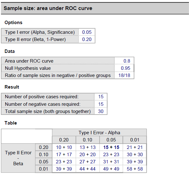 Fig. 18.
Power analysis test of the proposed aiGeneR model.
| Model | TP | FP | FN | TN |
| SVM | 5 | 2 | 1 | 6 |
| RF | 5 | 2 | 2 | 5 |
| XGBoost | 6 | 1 | 1 | 6 |
| ANN | 6 | 1 | 1 | 6 |
| aiGeneR | 7 | 0 | 1 | 6 |
Appendix E: Power Analysis
In the context of machine learning, power analysis often refers to the evaluation of the statistical power of the algorithms and experiments. It facilitates in determining whether your sample size is sufficient to identify any potential effects or relationships.
Appendix F: Selected Important Genes
Significant genes linked to antibiotic resistance in the context of urinary tract infections (UTIs) have been discovered by our AI model. These results provide critical information for developing antibiotic treatment plans and addressing UTI-related medication resistance. The aiGeneR-identified genes and their characteristics are detailed in Table 12.
| Gene Name | Importance |
| paaI | The phenylacetic acid breakdown pathway in E. coli includes the paaI gene. Phenylacetic acid can be broken down and used by the bacterium as a source of carbon and energy thanks to this route. Water and soil are two examples of natural habitats where phenylacetic acid can be found. E. coli can adapt to and endure situations where phenylacetic acid is present because of the paaI gene’s capacity to digest this substance [57]. |
| trpC | The tryptophan biosynthesis enzyme indole-3-glycerol phosphate synthase is encoded by the trpC gene in E. coli. E. coli is unable to synthesize tryptophan, an important amino acid. The trpC gene is essential for the bacteria to synthesize tryptophan on its own and meet its cellular needs for protein synthesis [58]. |
| polB | DNA polymerase II, commonly referred to as DNA polymerase IV (Pol IV), is encoded by the polB gene in E. coli. Enzymes called DNA polymerases are in charge of DNA replication, repair, and recombination. The polB gene produces the error-prone DNA polymerase DNA polymerase II, which participates in translesion synthesis (TLS) during DNA repair [59]. |
| pspB | Phage shock protein B (PspB), a subunit of the Phage shock protein (Psp) system, is produced by the pspB gene in E. coli. Under membrane stress, the Psp system, a stress response mechanism, aids E. coli cells in adapting and surviving [60]. |
| tetM | The Tet (M) protein, a well-known indicator of antibiotic resistance, is encoded by the tetM gene in E. coli. Tetracycline, a widely used antibiotic, becomes resistant to Tet(M). Through mobile genetic elements like plasmids or transposons, the tetM gene can be horizontally transferred between bacterial strains and species. This exchange may help bacterial populations, particularly E. coli, acquire tetracycline resistance. It is a serious issue in light of the spread of antibiotic resistance and the creation of multidrug-resistant microorganisms [61]. |
| The tetM gene frequently co-occurs with other genes for antibiotic resistance, such as those that confer resistance to different classes of antibiotics. This phenomenon of co-resistance might result via genetic linkage or co-selection, in which the use of one antibiotic favors the preservation of resistance genes for other antibiotics. Multidrug resistance in E. coli strains may be influenced by the tetM gene and other resistance factors. | |
| trpB | The tryptophan biosynthesis route includes the enzyme anthranilate synthase component I, which is encoded by the trpB gene in E. coli. Tryptophan, an important amino acid needed for protein synthesis and several biological functions, is produced by the trpB gene. An important step in the tryptophan biosynthesis route is the conversion of chorismate to anthranilate, which is catalyzed by the enzyme anthranilate synthase component I, which is encoded by trpB. E. coli is dependent on foreign supplies or the manufacture of tryptophan from precursors because it is unable to synthesize tryptophan on its own. The trpB gene and the enzymes it codes for are essential for ensuring that the cell has an adequate supply of tryptophan [62]. |
| adk | The adenylate kinase enzyme, which is encoded by the adk gene in E. coli, is essential for cellular energy metabolism. The equilibrium of adenine nucleotides, specifically ATP (adenosine triphosphate), ADP (adenosine diphosphate), and AMP (adenosine monophosphate), is maintained by adenylate kinase (adk). |
| ATP, ADP, and AMP are essential for energy transmission and utilization in a variety of cellular functions, and adenylate kinase aids in controlling their levels. It makes sure that the cell maintains a sufficient energy charge and ATP availability to support vital processes including cell motility, ion transport, and biosynthesis. To recycle nucleotides, adenylate kinase converts AMP and ADP back into ATP. This recycling procedure is crucial for the effective use of nucleotide pools and aids in the preservation of cellular resources [67, 68]. | |
| paaZ | Using crotonyl-CoA as a substrate, PaaZ displays enoyl-CoA hydratase activity. Exogenous Pseudomonas medium-chain-length polyhydroxyalkanoate synthase (PaaZ) generates (R)-3-hydroxyacyl-CoA for polyhydroxyalkanoate biosynthesis in a fadB mutant. A paaZ mutant shows a deficiency in using phenylacetate as a carbon source [69, 70]. |
Publisher’s Note: IMR Press stays neutral with regard to jurisdictional claims in published maps and institutional affiliations.